求解一元三次方程的原理与代码

本文记录了两种求解一元三次方程的方法：Cardano （卡丹）公式法和伴随矩阵特征值法。其中详细记录了 Cardano 公式的推导过程，以及使用三角函数对复数进行处理，避免复数运算的方法。然后简要介绍了多项式的伴随矩阵和通过伴随矩阵求特征值来获得根的方法。对各种方法分别给出了使用 C++ 以及 Python 求解单一方程和批量方程的代码。并尝试了使用 Pybind11 将 C++ 代码封装为 Python 模块再调用。最后对不同方法的求解速度进行了对比。文后还有一个彩蛋，介绍了 ChatGPT 给出的求解代码。

通过讨论发现，如果一次性已知大量方程的系数，通过 Cardano 公式使用向量化的 Python 代码求解的速度最快。如果必须通过循环才能获得方程的系数，无法使用向量化操作时，则通过 C++ 实现 Cardano 公式求解单一方程的函数，再封装成 Python 模块后调用的速度最快。本文的所有代码可在文末下载。

Cardano（卡丹）公式

推导过程

任意实系数一元三次方程：

\[ \begin{equation} a x^3 + b x^2 + c x + d = 0, a \neq 0 \end{equation} \]

都可以写为无二次项，三次项系数为 1 的形式：

\[ \begin{equation} y^3 + py + q = 0 \end{equation} \]

其中：

\[ \begin{equation} y = x + \frac{b}{3a}, \ p = \frac{3ac-b^2}{3a^2}, \ q = \frac{2b^3 - 9abc + 27a^2d}{27a^3} \end{equation} \]

Cardano 公式中构造两个新变量 \(u, v\) 使得：

\[ \begin{equation} u + v = y, \ 3uv + p = 0 \end{equation} \]

代入方程可得到

\[ \begin{equation} u^3 + v^3 = -q, \ uv = -\frac{p}{3} \end{equation} \]

可以发现，知道了 \(u^3, v^3\) 的和与积，则他们是下面关于 \(t\) 的二次方程的两个根：

\[ \begin{equation} t^2 + qt - \frac{p^3}{27} = 0 \end{equation} \]

解这个一元二次方程，令

\[ \begin{equation} \Delta = \frac{q^2}{4} + \frac{p^3}{27} \end{equation} \]

即一元二次方程判别式的 4 倍，则根据二次方程的求根公式，有：

\[ \begin{equation} u^3, v^3 = -\frac{q}{2} \pm \sqrt{\Delta} \end{equation} \]

代入原式发现只有当 \( u \neq v \) 时方程成立，则最终得到：

\[ \begin{equation} y = \sqrt[3]{-\frac{q}{2} - \sqrt{\frac{q^2}{4} + \frac{p^3}{27}}} + \sqrt[3]{-\frac{q}{2} + \sqrt{\frac{q^2}{4} + \frac{p^3}{27}}} \end{equation} \]

在 Cardano 公式诞生的时，还没有虚数的概念，因此这一公式就以这种形式表达。

复数域的解

引入复数之后，方程 \(w^3 = 1\) 的解有三个，分别是：

\[ \begin{equation} w_1=1, w_2=\frac{-1+\sqrt{3}i}{2}, w_3=\frac{-1-\sqrt{3}i}{2} \end{equation} \]

它们叫做三次单位根（third root of unity）。我们定义：

\[ \begin{equation} w = \frac{-1+\sqrt{3}i}{2} \end{equation} \]

式 (9) 中加号两边的立方根各有三个根，组合在一起共 9 个根。但是因为 \(u,v\) 的积需要满足式 (5) 中的关系，仅有三个根成立。他们是：

\[ \begin{equation} \begin{aligned} y_1 &= \sqrt[3]{R_1} + \sqrt[3]{R_2} \\ y_2 &= w\sqrt[3]{R_1} + w^2\sqrt[3]{R_2} \\ y_3 &= w^2\sqrt[3]{R_1} + w\sqrt[3]{R_2} \end{aligned} \end{equation} \]

由于 Python 的 numpy 库支持复数运算，所以使用这个公式可以直接在 Python 中获得复数解。

如果不想使用复数运算，则需要对判别式 \(\Delta\) 分类讨论。

当 \(\Delta = 0\) 时，公式可化简为：

\[ \begin{equation} y_1 = 2\sqrt[3]{-\frac{q}{2}}, y_2 = y_3 = -\sqrt[3]{-\frac{q}{2}} \end{equation} \]

方程有三个实根，其中有两个相等。

当 \(\Delta > 0\) 时，\(R_1, R_2\) 都是实数。如果把实部与虚部分开写，并记：

\[ \begin{equation} S = \sqrt[3]{R_1}, T=\sqrt[3]{R_2} \end{equation} \]

则有：

\[ \begin{equation} \begin{aligned} y_1 &= S + T \\ y_2 &= - \frac{1}{2}\left(S + T\right) + \frac{\sqrt{3}}{2}\left(S - T\right)i \\ y_3 &= - \frac{1}{2}\left(S + T\right) - \frac{\sqrt{3}}{2}\left(S - T\right)i \end{aligned} \end{equation} \]

三个解中一个为实数，另外两个为共轭复数。

但如果 \(\Delta < 0\) ，\(R_1, R_2\) 中对负数开平方，无法直接完成实部与虚部的分离。这时，可以借助三角函数来进一步分析。

使用三角函数分离实虚部

当 \( \Delta < 0 \) 时，有 \( p < 0 \)，则 \( R_1, R_2\) 是共轭复数。令：

\[ \begin{equation} -\frac{q}{2} \pm i\sqrt{-\Delta} = r(\cos{\varphi} \pm i\sin{\varphi}) \end{equation} \]

根据模相等，再根据实部相等，则有：

\[ \begin{equation} r = \sqrt{-\frac{p^3}{27}}, \ \cos{\varphi} = -\frac{q}{2r} \end{equation} \]

代入 Cardano 公式，得

\[ \begin{equation} y = 2 \sqrt[3]{r} \cos{\frac{\varphi + 2k\pi}{3}}, k=0,1,2 \end{equation} \]

有三个实根。

不仅当 \( \Delta < 0 \) 时可以使用三角函数处理，当 \( \Delta > 0 \) 也可以用以下方法处理。

（1）当 \( \Delta > 0, p < 0 \) 时，有：

\[ \begin{equation} 0 < \sqrt{-\frac{p^3}{27}} < \sqrt{\frac{q^2}{4}} = \frac{|q|}{2} \end{equation} \]

引进辅助角 \(\omega\) ：

\[ \begin{equation} \sqrt{-\frac{p^3}{27}} = \frac{q}{2} \sin{\omega}, \ \sqrt{\Delta} = \frac{q}{2}\cos{\omega} \end{equation} \]

则代入

\[ \begin{equation} \begin{aligned} \sqrt[3]{-\frac{q}{2} + \sqrt{\Delta}} = \sqrt[3]{-\frac{q}{2} + \frac{q}{2}\cos{\omega}} = -\sqrt{-\frac{p}{3}} \sqrt[3]{\tan{\frac{\omega}{2}}} \\ \sqrt[3]{-\frac{q}{2} - \sqrt{\Delta}} = \sqrt[3]{-\frac{q}{2} - \frac{q}{2}\cos{\omega}} = -\sqrt{-\frac{p}{3}} \sqrt[3]{\cot{\frac{\omega}{2}}} \end{aligned} \end{equation} \]

再引入角度：

\[ \begin{equation} \tan{\varphi} = \sqrt[3]{\tan{\frac{\omega}{2}}} \end{equation} \]

则有：

\[ \begin{equation} \tan{\varphi} + \cot{\varphi} = \frac{2}{\sin{2\varphi}} \end{equation} \]

令：

\[ \begin{equation} R_0 = -\frac{2\sqrt{-p/3}}{\sin{2\varphi}} \end{equation} \]

得到方程的三个根为：

\[ \begin{equation} \begin{aligned} y_1 &= R_0 \\ y_2 &= -\frac{R_0}{2} + \sqrt{-p}\cot{2\varphi}i \\ y_3 &= -\frac{R_0}{2} - \sqrt{-p}\cot{2\varphi}i \end{aligned} \end{equation} \]

（2）当 \( \Delta > 0, p > 0 \) 时，引进 \(\omega\)：

\[ \begin{equation} \sqrt{\frac{p^3}{27}} = \frac{q}{2}\tan{\omega}, \sqrt{\Delta} = \frac{q}{2}\frac{1}{\omega} \end{equation} \]

于是：

\[ \begin{equation} \begin{aligned} \sqrt[3]{-\frac{q}{2} + \sqrt{\Delta}} &= \sqrt[3]{\frac{q\sin^2{\left(\omega / 2\right)}}{\cos{\omega}}} = \sqrt{\frac{p}{3}} \cdot \sqrt[3]{\tan{\frac{\omega}{2}}} \\ \sqrt[3]{-\frac{q}{2} - \sqrt{\Delta}} &= -\sqrt[3]{\frac{q\cos^2{\left(\omega / 2\right)}}{\cos{\omega}}} = -\sqrt{\frac{p}{3}} \cdot \sqrt[3]{\cot{\frac{\omega}{2}}} \end{aligned} \end{equation} \]

再引进角度 \(\varphi\) ，使：

\[ \begin{equation} \tan{\varphi} = \sqrt[3]{\tan{\frac{\omega}{2}}} \end{equation} \]

则有方程的根：

\[ \begin{equation} \begin{aligned} y_1 &= \sqrt{\frac{p}{3}}\left(\tan{\varphi} - \cot{\varphi}\right) = -2\sqrt{\frac{p}{3}}\cot{2\varphi} \\ y_2 &= \sqrt{\frac{p}{3}} \cot{2\varphi} + \frac{\sqrt{p}}{\sin{2\varphi}}i \\ y_3 &= \sqrt{\frac{p}{3}} \cot{2\varphi} - \frac{\sqrt{p}}{\sin{2\varphi}}i \end{aligned} \end{equation} \]

小结

一次三次方程的根的情况为：当 \(\Delta < 0\) 时，有三个实根。当 \(\Delta > 0\) 时，有一个实根和两个共轭虚根。当 \(\Delta = 0\) 时，有三个实根，其中两个相等。

当 \(\Delta > 0\) 时，可以直接完成实虚部分离，也可以借助三角函数完成实虚部分离，前者相对简洁。当 \(\Delta < 0\) 时，需要借助三角函数完成实虚部分离。

综上，把公式总结起来，一元三次方程：

\[ \begin{equation} a x^3 + b x^2 + c x + d = 0, a \neq 0 \end{equation} \]

的解为：

\[ \begin{equation} \begin{aligned} x_0 &= -\frac{b}{3a} \\ p &= \frac{3ac-b^2}{3a^2}, \\ q &= \frac{2b^3 - 9abc + 27a^2d}{27a^3} \\ \Delta &= \frac{q^2}{4} + \frac{p^3}{27} \\ \textrm{If } \Delta \geq 0: \\ S &= \sqrt[3]{-\frac{q}{2} + \sqrt{\Delta}} \\ T &= \sqrt[3]{-\frac{q}{2} - \sqrt{\Delta}} \\ x_1 &= x_0 + S + T \\ x_2 &= x_0 - \frac{1}{2}\left(S + T\right) + \frac{\sqrt{3}}{2}\left(S - T\right)i \\ x_3 &= x_0 - \frac{1}{2}\left(S + T\right) - \frac{\sqrt{3}}{2}\left(S - T\right)i \\ \textrm{Else if } \Delta < 0: \\ r &= \sqrt{-\frac{p^3}{27}} \\ \varphi &= \arccos{\left(-\frac{q}{2r}\right)} \\ x_1 &= x_0 + 2 \sqrt[3]{r} \cos{\frac{\varphi}{3}} \\ x_2 &= x_0 + 2 \sqrt[3]{r} \cos{\frac{\varphi + 2\pi}{3}} \\ x_3 &= x_0 + 2 \sqrt[3]{r} \cos{\frac{\varphi + 4\pi}{3}} \end{aligned} \end{equation} \]

上式有一点需要注意，就是这里的三次根号是在实数范围内的，定义域和值域都是全体实数，且运算结果唯一。在编程时需要对符号进行处理。

代码实现

以下是一个 Cardano 公式的 C++ 函数的实现。将解得的三个根各用实部、虚部两个 double 类型保存，形成一个 6 维数组。

1
2
3
4
5
6
7
8
9
10
11
12
13
14
15
16
17
18
19
20
21
22
23
24
25
26
27
28
29
30
31
32
33
34
35
36
37
38
39
40
41
42
43
44
45
46
47
48
49
50
51
52
53
54
55
56
57

// In file cubicroot_cardano.cpp
#define M_PI 3.14159265358979323846

#include <cmath>
#include <iostream>

using namespace std;

void cubicSolve(double a, double b, double c, double d, double* roots)
{
    double p = (3 * a * c - b * b) / (3 * a * a);
    double q = (2 * b*b*b - 9 * a*b*c + 27 * a*a*d) / (27 * a*a*a);
    double discrim = (q * q) / 4 + (p * p * p) / 27;
    double x0 = - b / a / 3;
    double third = 1.0 / 3;
    double x1_real = 0.0;
    double x1_imag = 0.0;
    double x2_real = 0.0;
    double x2_imag = 0.0;
    double x3_real = 0.0;
    double x3_imag = 0.0;
    if (discrim > 0.0)
    {
        double s = - q / 2 + sqrt(discrim);
        s = ((s < 0) ? -pow(-s, third) : pow(s, third));
        double t = - q / 2 - sqrt(discrim);
        t = ((t < 0) ? -pow(-t, third) : pow(t, third));
        roots[0] = x0 + s + t;
        roots[1] = 0.0;
        roots[2] = x0 - (s + t) / 2;
        roots[3] = sqrt(3.0) * (s - t) / 2;
        roots[4] = roots[2];
        roots[5] = -roots[3];
    }
    else if (discrim < 0.0)
    {
        double r = sqrt(- p*p*p / 27);
        double phi = acos(-q / 2 / r);
        double rho = 2 * pow(r, third);
        roots[0] = x0 + rho * cos(phi / 3);
        roots[1] = 0.0;
        roots[2] = x0 + rho * cos((phi + 2.0 * M_PI) / 3.0);
        roots[3] = 0.0;
        roots[4] = x0 + rho * cos((phi + 4.0 * M_PI) / 3.0);
        roots[5] = 0.0;
    }
    else
    {
        double s = (q < 0) ? pow(-q / 2, third) : -pow(q / 2, third);
        roots[0] = x0 + 2 * s;
        roots[1] = 0.0;
        roots[2] = x0 - s;
        roots[3] = 0.0;
        roots[4] = roots[2];
        roots[5] = 0.0;
    }
}

同理，也可以使用以下 Python 代码来实现。源码来自这篇文章 。

1
2
3
4
5
6
7
8
9
10
11
12
13
14
15
16
17
18
19
20
21
22
23
24
25
26
27
28
29
30
31
32
33
34
35
36
37
38
39
40
41
42
43
44
45
46
47
48
49

import math

def cubic_solve(a0, b0, c0, d0):
    ''' Reduce the cubic equation to to form:
        x**3 + a*x**2 + b*x + c = 0 '''
    a, b, c = b0 / a0, c0 / a0, d0 / a0

    # Some repeating constants and variables
    third = 1. / 3.
    a13 = a * third
    a2 = a13 * a13
    sqr3 = math.sqrt(3)

    # Additional intermediate variables
    f = third * b - a2
    g = a13 * (2 * a2 - b) + c
    h = 0.25 * g * g + f * f * f

    def cubic_root(x):
        ''' Compute cubic root of a number while maintaining its sign'''
        if x.real >= 0:
            return x**third
        else:
            return -(-x)**third

    if f == g == h == 0:
        r1 = -cubic_root(c)
        return r1, r1, r1

    elif h <= 0:
        j = math.sqrt(-f)
        k = math.acos(-0.5 * g / (j * j * j))
        m = math.cos(third * k)
        n = sqr3 * math.sin(third * k)
        r1 = 2*j*m - a13
        r2 = -j * (m + n) - a13
        r3 = -j * (m - n) - a13
        return r1, r2, r3

    else:
        sqrt_h = math.sqrt(h)
        S = cubic_root(-0.5 * g + sqrt_h)
        U = cubic_root(-0.5 * g - sqrt_h)
        S_plus_U = S + U
        S_minus_U = S - U
        r1 = S_plus_U - a13
        r2 = -0.5 * S_plus_U - a13 + S_minus_U * sqr3 * 0.5j
        r3 = -0.5 * S_plus_U - a13 - S_minus_U * sqr3 * 0.5j
        return r1, r2, r3

在使用 python 的实现中，直接使用了 complex 数据类型来存储复数，运行函数直接返回三个根。

伴随矩阵特征值

计算原理

对于给定多项式函数：

\[ \begin{equation} P(x) = x^n + c_{n-1}x^{n-1} + c_{n-2}x^{n-2} + … + c_1 x + c_0 \end{equation} \]

其伴随矩阵（Companion Matrix）定义为：

\[ \begin{equation} M_x = \begin{pmatrix} 0 & 0 & \cdots & 0 & -c_0 \\ 1 & 0 & \cdots & 0 & -c_1 \\ 0 & 1 & \cdots & 0 & -c_2 \\ \vdots & \vdots & \ddots & \vdots & \vdots \\ 0 & 0 & \vdots & 1 & -c_{n-1} \end{pmatrix} \end{equation} \]

方程的根就是伴随矩阵的特征值。其简要证明可以在这篇文章找到。这种方式可以求任意次方程的根。

代码实现

求解矩阵的特征值是一个运算量比较大的工作，目前多数库都是调用 Fortran 为底层的 Lapack 工具箱来实现快速计算的。如果使用 C++ 迭代计算速度稍逊，如果使用 Python 迭代计算速度就更不用说了。因此这里不再写具体的矩阵求特征值方法，而是借助 C++ 的 Eigen 模块来完成。在下载之前，需要到其网站下载所需的头文件。在编译 C++ 时，需要使用 -I 标志指示编译器头文件的位置。

1
2
3
4
5
6
7
8
9
10
11
12
13
14
15
16
17
18
19
20

// In file: cubicroot_eigen.cpp
#include <Eigen/Dense>

void cubic_solve(double a, double b, double c, double d, double *roots)
{
    b = b / a;
    c = c / a;
    d = d / a;
    Eigen::Matrix3d m;
    m << 0, 0, -d,
         1, 0, -c,
         0, 1, -b;
    Eigen::Vector3cd es = m.eigenvalues();
    roots[0] = es[0].real();
    roots[1] = es[0].imag();
    roots[2] = es[0].real();
    roots[3] = es[0].imag();
    roots[4] = es[0].real();
    roots[5] = es[0].imag();
}

这里使用了与上节相同的函数头，把结果用 6 个值的数组保存。实际上也可以直接返回 Vector3cd 类型的数据。

下面是一段使用 Python 来实现的代码，使用了 numpy 库。

1
2
3
4
5
6
7
8
9
10

# In file: cubicroot_eigen.py
import numpy as np

def solve_cubic(a, b, c, d):
	
    b = b / a
    c = c / a
    d = d / a
    M = np.array([[0., 0., -d], [1., 0., -c], [0., 1., -b]])
    return np.linalg.eigvals(M)

批量计算

如果有大量方程需要一次性求解，在 C++ 中可以通过循环完成。而在 Python 中，如果使用 for 循环，效率非常低，需要使用向量化操作，才能大幅提升性能。这里参考这篇文章给出使用 Cardano 公式批量求解的代码：

1
2
3
4
5
6
7
8
9
10
11
12
13
14
15
16
17
18
19
20
21
22
23
24
25
26
27
28
29
30
31
32
33
34
35
36
37
38
39
40
41
42
43
44
45
46
47
48
49
50
51
52
53
54
55
56
57
58
59
60
61
62
63
64
65
66
67
68
69
70
71
72
73
74
75
76
77
78
79
80
81
82
83
84
85
86
87

# In file: cubicroot_cardano_python.py
import numpy as np
import math

def multi_cubic(a0, b0, c0, d0, all_roots=True):
    # Cubic coefficients
    a, b, c = b0 / a0, c0 / a0, d0 / a0

    # Some repeating constants and variables
    third = 1.0 / 3.0
    a_third = a * third
    a_third_square = a_third * a_third
    sqr3 = math.sqrt(3)

    # Additional intermediate variables
    f = third * b - a_third_square
    g = a_third * (2 * a_third_square - b) + c
    h = 0.25 * g * g + f * f * f

    # Masks for different combinations of roots
    m1 = (f == 0) & (g == 0) & (h == 0)     # roots are real and equal
    m2 = (~m1) & (h <= 0)                   # roots are real and distinct
    m3 = (~m1) & (~m2)                      # one real root and two complex

    def cubic_root(x):
        ''' Compute cubic root of a number while maintaining its sign
        '''
        root = np.zeros_like(x)
        positive = (x >= 0)
        negative = ~positive
        root[positive] = x[positive] ** third
        root[negative] = -(-x[negative]) ** third
        return root

    def roots_all_real_equal(c):
        ''' Compute cubic roots if all roots are real and equal
        '''
        r1 = -cubic_root(c)
        if all_roots:
            return r1, r1, r1
        else:
            return r1

    def roots_all_real_distinct(a13, f, g, h):
        ''' Compute cubic roots if all roots are real and distinct
        '''
        j = np.sqrt(-f)
        k = np.arccos(-0.5 * g / (j * j * j))
        m = np.cos(third * k)
        r1 = 2 * j * m - a13
        if all_roots:
            n = sqr3 * np.sin(third * k)
            r2 = -j * (m + n) - a13
            r3 = -j * (m - n) - a13
            return r1, r2, r3
        else:
            return r1

    def roots_one_real(a13, g, h):
        ''' Compute cubic roots if one root is real and other two are complex
        '''
        sqrt_h = np.sqrt(h)
        S = cubic_root(-0.5 * g + sqrt_h)
        U = cubic_root(-0.5 * g - sqrt_h)
        S_plus_U = S + U
        r1 = S_plus_U - a13
        if all_roots:
            S_minus_U = S - U
            r2 = -0.5 * S_plus_U - a13 + S_minus_U * sqr3 * 0.5j
            r3 = -0.5 * S_plus_U - a13 - S_minus_U * sqr3 * 0.5j
            return r1, r2, r3
        else:
            return r1

    # Compute roots
    if all_roots:
        roots = np.zeros((3, len(a))).astype(complex)
        roots[:, m1] = roots_all_real_equal(c[m1])
        roots[:, m2] = roots_all_real_distinct(a_third[m2], f[m2], g[m2], h[m2])
        roots[:, m3] = roots_one_real(a_third[m3], g[m3], h[m3])
    else:
        roots = np.zeros(len(a))
        roots[m1] = roots_all_real_equal(c[m1])
        roots[m2] = roots_all_real_distinct(a_third[m2], f[m2], g[m2], h[m2])
        roots[m3] = roots_one_real(a_third[m3], g[m3], h[m3])

    return roots

这里使用了 mask 来避免用 if 判断，可以提高运算速度。

还有使用特征值法向量化求解的 Python 代码：

1
2
3
4
5
6
7
8
9
10
11
12
13
14
15

# In file: cubicroot_eigen_multi.py
import numpy as np

def solve_cubic_multi(p):
	
    # Coefficients of quartic equation
    a, b, c = p[:, 1]/p[:, 0], p[:, 2]/p[:, 0], p[:, 3]/p[:, 0]
	
    # Construct the companion matrix
    A = np.zeros((len(a), 3, 3))
    A[:, 1:, :2] = np.eye(2)
    A[:, :, 2] = -np.array([c, b, a]).T
	
    # Compute roots using eigenvalues
    return np.linalg.eigvals(A)

这里在构建伴随矩阵时，使用了三阶张量。可以一次性求解大批量特征值。

C++ 封装为 Python 模块

使用 Python 与 C++ 对比运行时间不太公平，因为 Python 牺牲了一些速度换来的是极大的便利。下面我们把 C++ 写的函数封装成 Python 模块，再来对比时间。

在 加快 Python 调用 OpenSees 的速度 一文中，我已经介绍了使用原生方法在 Linux 中把 C++ 代码封装成动态链接库，再在 Python 中直接 import 的方法。它通过 Python.h 头文件中定义的 PyModuleDef PyMethodDef PyMODINIT_FUNC 等函数和类型来完成封装。

本文介绍另一种方法，使用现在比较流行的 Pybind11 来完成封装工作。

安装 Pybind11

安装的方法有很多，由于我使用的是 Anaconda ，可以直接通过 conda-forge 来安装：

1

conda install -c conda-forge pybind11

此外还需要安装 C++ 的生成工具。如果上文的 C++ 代码可以成功编译，说明已经安装好了 C++ 的生成工具。这里我使用的是 Visual Studio 提供的 MSVC 来构建。这样就不用在 Windows 中再来安装 g++ 了。

MSVC 提供了 cl.exe link.exe 来完成编译，使用方法与 g++ 类似，只是参数的输入方法有所不同。要在终端使用 cl.exe 的话，需要打开 Visual Studio 提供的终端，它会自动设置一些编译所需的环境变量。具体的编译方法可以参考这篇文章。但使用 Pybind11 时不需要我们手动编译，它提供的 extension 可以自动找到系统中的编译器并进行编译，在后文中会提到。但是编写 C++ 函数时需要编译和测试。

写封装用的 C++ 函数

首先创建一个文件夹，命名为 mycubicmodule ，后面把我们编写的模块所需文件都放在这个文件夹里。其结构如下：

1
2
3
4
5

mycubicmodule
    bind.cpp
    cubicroot.cpp
    pyproject.toml
    setup.py

其中 cubicroot.cpp 是把前文中 cubicroot_cardan.cpp 这一文件重命名后复制过来的。 bind.cpp 定义了原 C++ 文件与 Python 交互所用的函数，代码如下：

1
2
3
4
5
6
7
8
9
10
11
12
13
14
15
16
17
18
19
20
21
22
23
24
25
26
27
28
29
30
31
32
33
34
35
36
37
38
39

// in mycubicmodule/bind.cpp
#include <iostream>
#include <pybind11/pybind11.h>
#include <pybind11/stl.h>
#include <vector>

void cubicSolve(double a, double b, double c, double d, double* roots);

namespace py = pybind11;
using namespace std;

vector<double> cubicSolveSingle(double a, double b, double c, double d)
{
    double roots[6];
    cubicSolve(a, b, c, d, roots);
    vector<double> result(roots, roots + 6);
    return result;
}

vector<vector<double>> cubicSolveMultiple(vector<vector<double>> &&coeffs)
{
    size_t size = coeffs.size();
    vector<vector<double>> result;
    result.reserve(size);
    double roots[6];
    for (vector<double> & c : coeffs)
    {
        cubicSolve(c[0], c[1], c[2], c[3], roots);
        vector<double> roots_vec(roots, roots + 6);
        result.push_back(roots_vec);
    }
    return result;
}

PYBIND11_MODULE(mycubicmodule, m) {
    m.doc() = "";
    m.def("cubic_solve", &cubicSolveSingle, "");
    m.def("cubic_solve_multi", &cubicSolveMultiple, "");
}

使用 std::vector 类型将返回值封装起来， Pybind11 可以自动识别，并与 Python 中的 list 类型对应。

编写安装文件

在 pyproject.toml 中，根据 PEP 517 的规定，可以定义在使用 pip 安装模块时，安装之前需要加载的模块。这里除了需要使用 setuptools 以外，还需要使用 pybind11 。有了这个文件， pip 在安装模块之前，会自动先安装这两个库，作为我们安装时的依赖项。

1
2
3
4
5
6

[build-system]
requires = [
    "setuptools>=42",
    "pybind11>=2.10.0",
]
build-backend = "setuptools.build_meta"

最后是在 setup.py 中定义安装所需的代码：

1
2
3
4
5
6
7
8
9
10
11
12
13
14
15
16
17
18
19
20
21
22
23
24
25
26
27
28

import sys

# Available at setup time due to pyproject.toml
from pybind11 import get_cmake_dir
from pybind11.setup_helpers import Pybind11Extension, build_ext
from setuptools import setup

__version__ = "0.0.1"

ext_modules = [
    Pybind11Extension("mycubicmodule",
        ["bind.cpp", "cubicroot.cpp"],
    ),
]

setup(
    name="mycubicmodule",
    version=__version__,
    author="Hanlin Dong",
    author_email="self@hanlindong.com",
    url="http://www.hanlindong.com/2023/cubic-equation/",
    description="Solve cubic equation module",
    long_description="",
    ext_modules=ext_modules,
    cmdclass={"build_ext": build_ext},
    zip_safe=False,
    python_requires=">=3.7",
)

编译安装

以上文件准备好后，即可开始编译。注意计算机中需要有 C++ 编译器，可以使用 Visual Studio 提供的 MSVC 编译器，也可以使用 g++ 等编译器。 Pybind11 会自动在系统中搜索可用的编译器。打开终端，切入 mycubicmodule 文件夹所在的目录，再输入

1

pip install ./mycubicmodule

可以看到程序开始自动安装 setuptools 和 pybind11 。安装好后就会使用编译器进行编译，编译的 warning 等信息都会同样打印到控制台。完成之后，输入

1

pip show mycubicmodule

即可看到这个库的信息。

运行时间对比

这里对使用 Cardano 公式求解、使用伴随矩阵特征值求解，以及使用 numpy 求解一万个三次方程的速度进行对比。

首先是记录 C++ 求解时间的函数：

1
2
3
4
5
6
7
8
9
10
11
12
13
14
15
16
17
18
19
20
21
22
23
24
25
26
27
28
29

// in cubicroot_cardano.cpp and cubicroot_eigen.cpp
double getTime() 
{
    const long COUNT = 10000;
    double x[COUNT * 3];
    double r[COUNT * 6];
    srand(time(NULL));
    for (long i = 0; i < COUNT * 3; i++) {
        x[i] = rand() * 2;
    }
    clock_t start_time, end_time;
    start_time = clock();
    double roots[6];
    for (long j = 0; j < COUNT; j++) {
        cubicSolve(1.0, x[j*3], x[j*3+1], x[j*3+2], roots);
        for (long i = 0; i < 6; i++) {
            r[j*6+i] = roots[i];
        }
    }
    end_time = clock();
    return (double)(end_time - start_time) / CLOCKS_PER_SEC;
}

int main()
{
    double t = getTime();
    cout << "Time to solve the cubic equations: " << t * 1000 << " ms" << endl;
    return 0;
}

运行 7 次，使用 Cardano 公式求解的平均时间为：1 ms 。使用 Eigen 求解的平均时间为：501 ms 。可见使用 Cardano 公式计算时间非常短。这与 Eigen 求解器使用了比较复杂的数据结构可能也有关系。实际上，使用 clock() 来记录时间的精度不是很高，实际上 Cardano 公式求解的执行时间可能小于 1 ms。

再来看使用 Python 来计算的结果。用 ipython 中的 %%timeit 来记录时间：

1
2
3
4
5
6
7
8
9
10
11
12
13
14
15
16
17
18
19
20
21
22
23
24
25
26
27
28
29
30
31
32

# %%
import numpy as np
from numpy.polynomial.polynomial import Polynomial
from cubicroot_eigen_multi import cubic_solve_multi as csm_eigen
from cubicroot_cardano import cubic_solve as cubic_solve_py
from cubicroot_cardano_multi import cubic_solve_multi as csm_cardano
from mycubicmodule import cubic_solve as cubic_solve_cpp
from mycubicmodule import cubic_solve_multi as csm_cpp

# %%
num_equations = 10000
# Generate some random coefficients
coeffs = np.random.rand(num_equations, 3) * 2
coeffs = np.hstack([np.ones(num_equations).reshape(-1, 1), coeffs])
# reverse for polynomial constructor
coeffs2 = np.vstack([coeffs[:, 3], coeffs[:, 2], coeffs[:, 1], coeffs[:, 0]]).T

# %%
print("Time using `numpy.roots`:")
%timeit root1 = [np.roots(coeff) for coeff in coeffs]
print("Time using `Polynomial.roots`:")
%timeit root2 = [Polynomial(coeff).roots() for coeff in coeffs2]
print("Time using python function solving multiple eigen values vectorized:")
%timeit root3 = csm_eigen(coeffs)
print("Time using python Cardano formula individually:")
%timeit root4 = [cubic_solve_py(*coeff) for coeff in coeffs]
print("Time using python Cardano formula vectorized:")
%timeit root5 = csm_cardano(*coeffs.T)
print("Time using C++ Cardano formula individually:")
%timeit root6 = [cubic_solve_cpp(*coeff) for coeff in coeffs]
print("Time using C++ looped Cardano formula:")
%timeit root7 = csm_cpp(coeffs)

得到的结果如下：

1
2
3
4
5
6
7
8
9
10
11
12
13
14

Time using `numpy.roots`:
339 ms ± 9.82 ms per loop (mean ± std. dev. of 7 runs, 1 loop each)
Time using `Polynomial.roots`:
436 ms ± 11.7 ms per loop (mean ± std. dev. of 7 runs, 1 loop each)
Time using python function solving multiple eigen values:
10.9 ms ± 319 µs per loop (mean ± std. dev. of 7 runs, 100 loops each)
Time using python Cardano formula individually:
112 ms ± 918 µs per loop (mean ± std. dev. of 7 runs, 10 loops each)
Time using python Cardano formula vectorized:
1.9 ms ± 25.4 µs per loop (mean ± std. dev. of 7 runs, 1,000 loops each)
Time using C++ Cardano formula individually:
15.6 ms ± 62 µs per loop (mean ± std. dev. of 7 runs, 100 loops each)
Time using C++ looped Cardano formula:
5.78 ms ± 119 µs per loop (mean ± std. dev. of 7 runs, 100 loops each)

可见最快的是使用向量化 Cardano 公式的 python 函数，平均 1.9 ms 即计算完成。其次是在 C++ 中循环使用 Cardano 公式的函数，平均 5.78 ms 计算完成。再次是 Python 中使用向量化的求特征值方法，平均时间为 10.9 ms 。然后是使用 C++ 单次计算 Cardan 公式，并在 Python 中完成循环，平均时间为 15.6 ms 。其余方法的时间都相对较长。

综上，在一次性知道大批量方程的系数时，使用向量化的 Cardano 公式的运算速度最快。如果一次只知道一个方程的系数，必须通过循环来计算的话，使用 C++ 实现的 Cardano 公式计算比使用 Python 实现的 Cardano 公式计算的效率更高，提升约 7 倍。

彩蛋：咨询 ChatGPT

下面我们来问问 OpenAI 的 ChatGPT ，看他有什么想法，见下图：

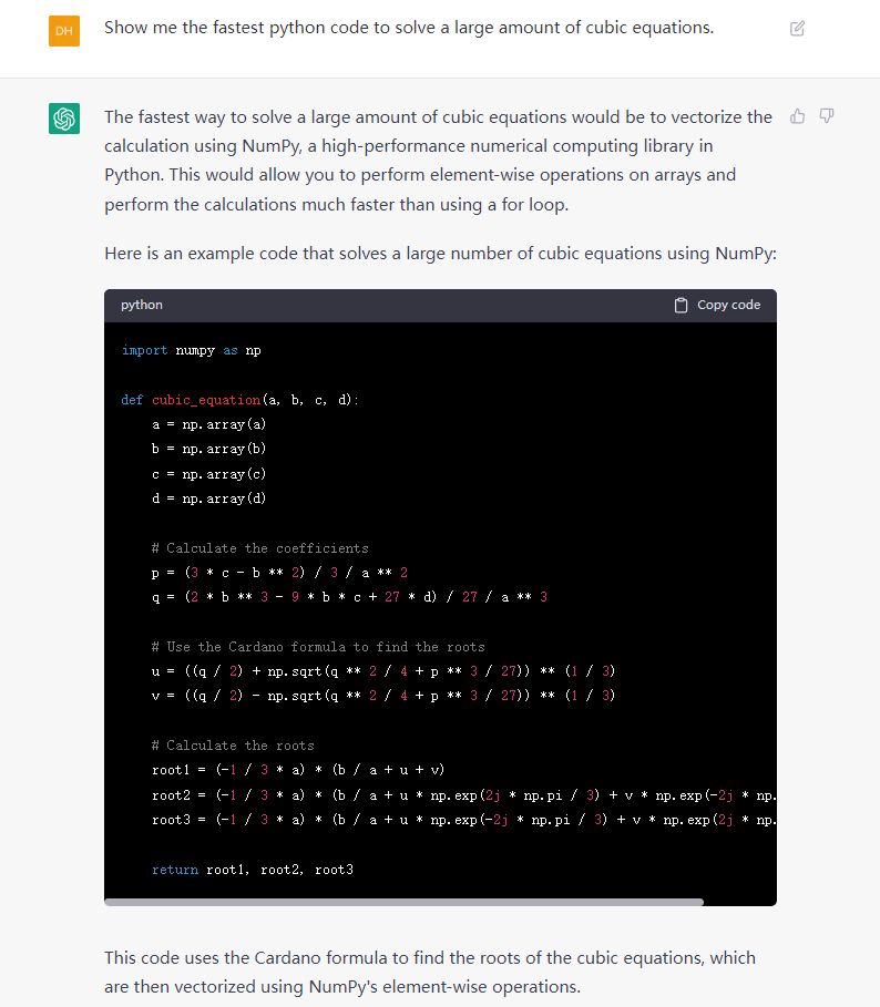
可见 ChatGPT 准确地给出了我们刚才讨论的最快方法。把这个函数保存为 chatgpt_suggestion.py ，运行会发现，得出的结果并不正确。也就是说，ChatGPT 依葫芦画瓢给出的代码很像 Cardano 公式，但是实际上并不是准确的 Cardano 公式，不能直接使用。但是它给了一个思路，就是可以直接使用 numpy 的复数运算功能套用 Cardano 公式，而无需分类做各种处理。这是在前文中没有想到的。下面我对 ChatGPT 给出的代码给出评论，再更正为正确的代码。

1
2
3
4
5
6
7
8
9
10
11
12
13
14
15
16
17
18
19
20
21
22
23
24
25
26
27
28
29
30
31
32
33
34
35
36
37
38
39
40
41
42
43
44
45
46
47
48
49
50
51
52
53
54
55

# In file: chatgpt_suggestion.py
import numpy as np

def cubic_equation(a, b, c, d):
    a = np.array(a)
    b = np.array(b)
    c = np.array(c)
    d = np.array(d)

    # Calculate the coefficients
    # 注：以下 p 和 q 的计算公式有几项漏掉了 a ，
    # 这很可能是因为在某些代码中对 a 进行了归一化，但某些没有，ai 看不懂了。
    p = (3 * c - b ** 2) / 3 / a ** 2
    q = (2 * b ** 3 - 9 * b * c + 27 * d) / 27 / a ** 3

    # Use the Cardano formula to find the roots
    # 注：`np.sqrt` 不能直接对负数运算，会得到 NaN 。要使用 `np.emath.sqrt`。
    # 负数也不能开三次方，要处理符号。
    u = ((q / 2) + np.sqrt(q ** 2 / 4 + p ** 3 / 27)) ** (1 / 3)
    v = ((q / 2) - np.sqrt(q ** 2 / 4 + p ** 3 / 27)) ** (1 / 3)

    # Calculate the roots
    # 注：下面的公式看上去有些问题，似乎没有把 3a 作为整体分母的表达方式。计算结果是错误的。
    root1 = (-1 / 3 * a) * (b / a + u + v)
    root2 = (-1 / 3 * a) * (b / a + u * np.exp(2j * np.pi / 3) + v * np.exp(-2j * np.pi / 3))
    root3 = (-1 / 3 * a) * (b / a + u * np.exp(-2j * np.pi / 3) + v * np.exp(2j * np.pi / 3))

    return root1, root2, root3

def cubic_equation_corrected(a, b, c, d):
    a = np.array(a)
    b = np.array(b)
    c = np.array(c)
    d = np.array(d)

    # Calculate the coefficients
    p = (3 * a * c - b ** 2) / 3 / a ** 2
    q = (2 * b ** 3 - 9 * a * b * c + 27 * a ** 2 * d) / 27 / a ** 3

    # Use the Cardano formula to find the roots
    delta = q ** 2 / 4 + p ** 3 / 27
    u3 = - q / 2 - np.emath.sqrt(delta)
    v3 = - q / 2 + np.emath.sqrt(delta)
    u = np.sign(u3) * np.abs(u3) ** (1 / 3)
    v = np.sign(v3) * np.abs(v3) ** (1 / 3)

    # Calculate the roots
    x0 = - b / 3 / a
    w = (-1 + np.sqrt(3) * 1j) / 2
    w2 = w ** 2
    root1 = x0 + u + v
    root2 = x0 + w * u + w2 * v
    root3 = x0 + w2 * u + w * v

    return root1, root2, root3

1
2
3
4
5
6
7
8

# %%
from chatgpt_suggestion import cubic_equation_corrected as chatgpt_solver

# %%
print("Time using ChatGPT suggested direct solver:")
%timeit root8 = [chatgpt_solver(*coeff) for coeff in coeffs]
print("Time using ChatGPT suggested direct solver vectorized:")
%timeit root9 = chatgpt_solver(*coeffs.T)

结果为：

1
2
3
4

Time using ChatGPT suggested direct solver:
402 ms ± 9.21 ms per loop (mean ± std. dev. of 7 runs, 1 loop each)
Time using ChatGPT suggested direct solver vectorized:
2.08 ms ± 91.6 µs per loop (mean ± std. dev. of 7 runs, 100 loops each)

可见向量化运算的速度与我们上文所发现的最快方法所差无几。同时，它直接利用了 numpy 中对负数开根号的运算，代码看起来更简洁。可见 ChatGPT 还是很强大的，只是生成的代码还需要一定的手工更正。

P.S. 也许是运气比较好，第一次问 ChatGPT 就得到了想要的答案。但我发现应该是用 a large number of equations ，而不是用 amount 。但是换用其它词问 ChatGPT 时，很难再得出直接使用 Cardano 公式计算的代码，多数是给使用 np.root 及 scipy.optimize 中的迭代方法等求解。另外，我还尝试了要求 ChatGPT 自行对上面的代码进行更正并加上单元测试，但它似乎没有这个能力。另外 GPT3 还有专门生成代码用的子集 Codex ，目前还不是很好用。我们拭目以待！

以上讨论的代码可以点此下载。

参考文献：

1. 华罗庚. 高等数学引论（第一册）. 高等教育出版社. 2009.
2. Nino Krvavica. On computing roots of quartic and cubic equations in Python. Personal website. 2019. https://nkrvavica.github.io/post/on_computing_roots/
3. Mathis Wang. 一元三次方程的求根公式. 知乎专栏：数学学习笔记. 2023. https://zhuanlan.zhihu.com/p/137077558
4. Jinyu Li. 多项式的伴随矩阵. Personal website. 2016. https://jinyu.li/2016/12/04/companion-matrix/
5. 苏建林. 三次方程的三角函数解法. 科学空间网站. https://www.spaces.ac.cn/archives/831
6. Wikipedia. Cubic equation. Wikipedia website. https://en.wikipedia.org/wiki/Cubic_equation
7. Weisstein, Eric W. Cubic Formula. From MathWorld–A Wolfram Web Resource. https://mathworld.wolfram.com/CubicFormula.html
8. BaseMax. Cubic Equation Calculator. Github repository. https://github.com/BaseMax/CubicEquationCalculator