本文使用 OpenSees 来完成结构动力学中与单自由度体系(SDOF)有关的动力分析。
1 | import openseespy.opensees as ops |
SDOF 静力分析
在动力分析之前,先熟悉 SDOF 体系的建模和静力分析方法。使用弹簧-小车模型建模,分别进行力控制和位移控制的分析。
1 | # 单自由度体系静力分析 - 力控制 |
1.8571428571428568
以上代码定义了一个刚度 \(K=7\) 的弹簧,加了 \(F=13 \) 的外荷载,输出位移为 \(\Delta = F / K = 1.8571 \) ,与 OpenSees 的输出相同。
下面我们来进行位移控制的加载。
1 | # 单自由度体系静力分析 - 位移控制 |
Force1: -6.999999999999999
Force2: 6.999999999999998
以上使用位移控制加载,通过 10 步完成了目标位移为 1 的加载。最后在输出时,通过两种方式完成。第一是通过读取 twoNodeLink 单元的内力来完成。此时输出的是一个负值。表示这个单元的左侧节点对单元的作用力是向左的。第二是通过读取 time ,再乘以 load 中的数值 13 完成的。这是因为定义了一个 Linear 类型的 timeSeries ,且比例因子为默认的 1 。此时将 time 与 load 相乘,即为结构当前所受的外荷载。
SDOF 自由振动
下面我们来分析 SDOF 体系的自由振动。为使体系自由振动起来,需要给结构一个初始扰动。这里有两种方式,第一是先通过 pattern 加一个初始力,然后再移除初始力,进行动力分析。第二是直接在定义节点的时候,给一个初始的位移。我们用第一种方式来计算一个无阻尼自由振动,再用第二种方式计算一个有阻尼自由振动。
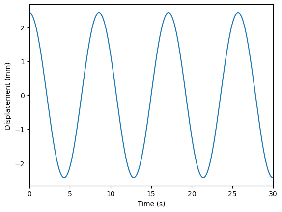
无阻尼自由振动
1 | # SDOF自由振动 - 先施加力再卸掉 |
WARNING analysis Transient - no Integrator specified,
 TransientIntegrator default will be used
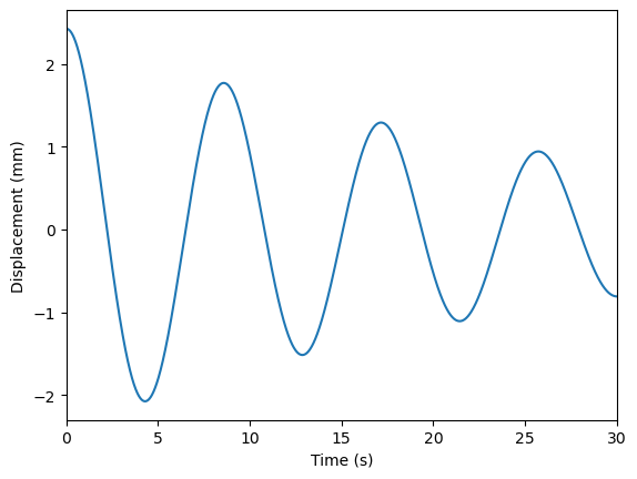
有阻尼自由振动
下面我们使用直接加初始位移的方式来施加初始扰动。然后使用 OpenSees 中的 Rayleigh 命令来施加阻尼。
对于单自由度体系,Rayleigh 阻尼中的质量系数和刚度系数任取其一即可。这里我们使用质量系数。则有
$$ c = 2 m \zeta \omega = \alpha m $$
则
$$ \alpha = 2 \zeta \omega $$
1 | # SDOF有阻尼自由振动 - 直接加初始位移 |
WARNING - the 'fullGenLapack' eigen solver is VERY SLOW. Consider using the default eigen solver.

Omega:  0.7337993857053428
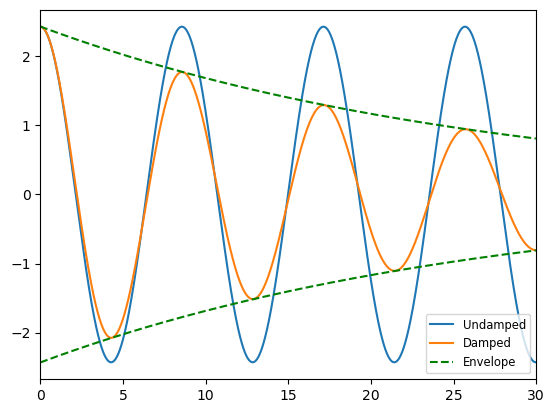
根据响应计算自振特性
下面我们将有、无阻尼的响应画在一起,并画出有阻尼结构振动的包络线。包络线的表达式为
$$ u = \rho e^{ - \zeta \omega_{n} t} $$
其中
$$ \rho = \sqrt{u_0^2 + \left(\frac{\dot{u_0} + \zeta \omega_n u_0}{\omega_D}\right)^2} $$
代入数据
$$ \omega_n = \sqrt{\frac{k}{m}} = \frac{7}{13} = 0.7338 $$
$$ \omega_D = \omega_n \sqrt{1-\zeta^2} = 0.7338 * \sqrt{1-0.05^2} = 0.7329 $$
$$ u_0 = 17 / 7 = 2.4286 $$
$$ \dot{u_0} = 0 $$
$$ \rho = \sqrt{ 2.4286^2 + \left(\frac{0.05 \times 0.7329 \times 2.4286 }{0.7338}\right)^2} = 2.4316 $$
根据上述计算可以输出包络线,代码如下
1 | plt.figure() |
<matplotlib.legend.Legend at 0x235043f4400>
下面我们来根据响应计算结构的周期和阻尼比。首先找到输出曲线的极值点,并取第一个和第三个进行计算。
1 | from scipy import signal |
Undamped period:  8.56
Damped period:  8.57
Damping ratio:  0.05006255873633257
再根据结构定义进行计算
$$ T_n = \frac{2\pi}{\omega_n} = 8.5625 \mathrm{s} $$
$$ T_d = T_n / \sqrt{1-\zeta^2} = 8.5732 \mathrm{s} $$
可见结果基本吻合。
SDOF 受迫振动-简谐荷载
无阻尼
下面进行 SDOF 体系的受迫振动分析。首先对静止的无阻尼的结构施加简谐荷载。
1 | # 无阻尼SDOF受迫振动 - 简谐荷载 |
Omega: 0.7337993857053428
可见无阻尼 SDOF 在简谐波的作用下,响应为自由振动与外力引起的振动叠加。
共振现象
当外荷载的周期接近结构的自振周期时,会出现共振现象。让我们来尝试一下。将外加简谐荷载的周期调整为 8.56 s:
1 | # 无阻尼SDOF受迫振动 - 简谐荷载 - 共振 |
Omega: 0.7337993857053428
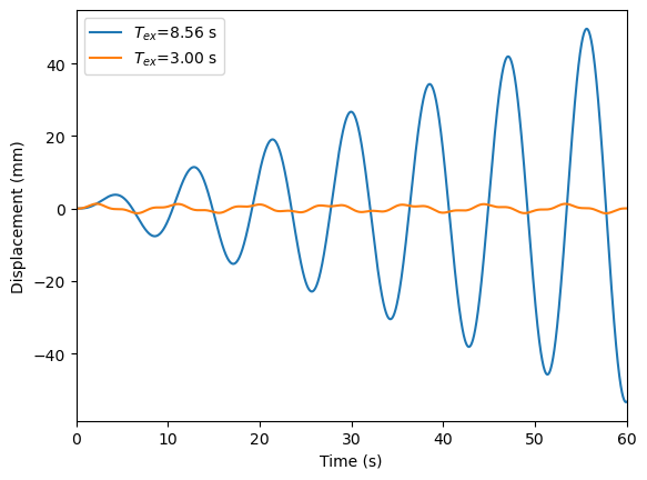
可见发生共振时,结构的振动幅值不断增大。
有阻尼
下面给结构加上阻尼,再来观察结果。
1 | # 有阻尼SDOF受迫振动 - 简谐荷载 |
Omega:  0.7337993857053428
Omega:  0.7337993857053428
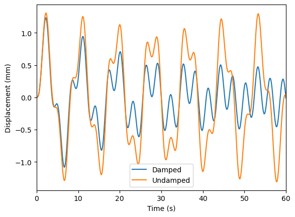
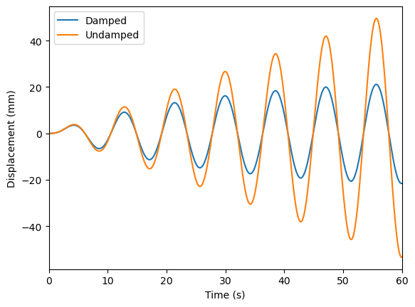
以上两张图,从上面一张可以看出,对于有阻尼结构,其自由振动会逐渐耗散,振动的频率渐渐地与外荷载的频率相同。当外荷载的频率与自振频率接近时,结构发生共振,但是有阻尼结构的振幅不会发散,而是稳定在一个常数。该常数约等于 \( 1/2 \zeta u_{st} \)。
值得注意的是,在使用 eigen 命令输出特征值时,无论结构是否定义了阻尼,输出的都是无阻尼的特征值,即 \(\omega_n\) 。对于有阻尼体系,需要有阻尼特征值 \(\omega_D\) 时,需要自行计算。
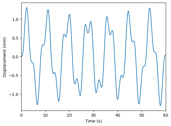
SDOF 地震作用
SDOF 在地震作用下的响应
在地震工程研究中,常常需要分析 SDOF 在地震作用下的响应。这里可以使用 OpenSees 的 UniformExcitation 来完成。下面我们来分析一个有阻尼 SDOF 在 El Centro 波下的响应。 El Centro 波的时程可以在 这里下载。需要把解压得到的 accel.txt 文件放在工作目录中。注意这个文件中共3000个点,采样时间间隔为 0.01s,加速度的单位为 g 。
1 | # 有阻尼 SDOF 在地震作用下的响应 |
Omega:  2.23606797749979
Period:  2.808501379739736
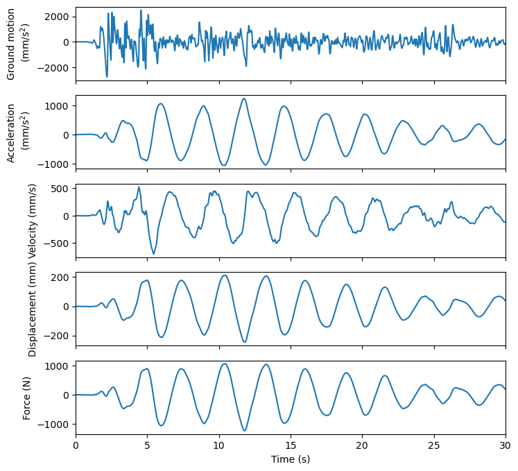
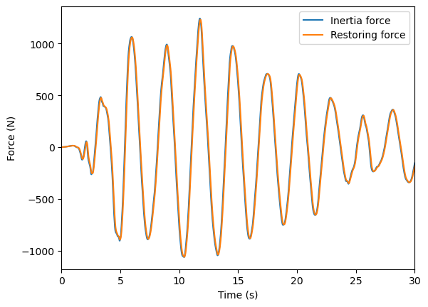
从图中可以看出,结构的加速度、位移、内力时程的形状基本是一样的,只差一个系数。内力和加速度的相反数之比为结构质量,内力和位移之比为结构刚度。注意惯性力并不完全与内力相等,它们之间相差一个阻尼力。因为阻尼力很小,可近似认为它们相等。我们把惯性力和内力画在一起做个比较:
1 | plt.figure() |
基于 SDOF 画反应谱
下面我们借助 OpenSees ,批量建立 SDOF 结构并求其响应,从而绘制反应谱。
1 | def peakResponse(period, damping=0.05, accel_file="accel.txt"): |
1 | plt.figure(figsize=(4, 3)) |
(0.0, 0.2628783530740493)
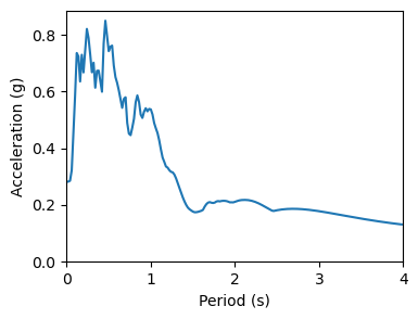
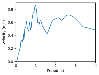
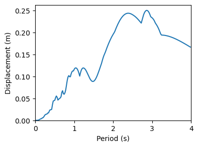
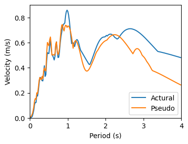
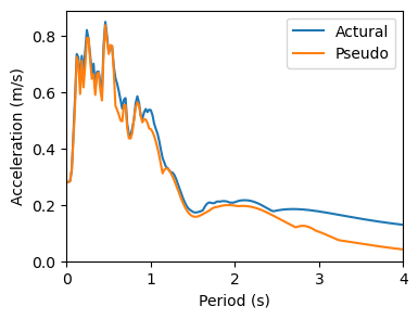
实际上,可以通过将位移反应谱乘以 \(\omega\) 得到伪速度反应谱,再乘以 \(\omega\) 得到伪位移反应谱。我们来比较一下:
1 | plt.figure(figsize=(4, 3)) |
C:\Users\hanlin\AppData\Local\Temp\ipykernel_15968\2916255756.py:3: RuntimeWarning: divide by zero encountered in true_divide
  plt.plot(periods, np.array(disps) * (2 * np.pi / periods) / 1000, label="Pseudo")
C:\Users\hanlin\AppData\Local\Temp\ipykernel_15968\2916255756.py:3: RuntimeWarning: invalid value encountered in multiply
  plt.plot(periods, np.array(disps) * (2 * np.pi / periods) / 1000, label="Pseudo")
C:\Users\hanlin\AppData\Local\Temp\ipykernel_15968\2916255756.py:12: RuntimeWarning: divide by zero encountered in true_divide
  plt.plot(periods, np.array(disps) * (2 * np.pi / periods) ** 2 / 9800, label="Pseudo")
C:\Users\hanlin\AppData\Local\Temp\ipykernel_15968\2916255756.py:12: RuntimeWarning: invalid value encountered in multiply
  plt.plot(periods, np.array(disps) * (2 * np.pi / periods) ** 2 / 9800, label="Pseudo")


<matplotlib.legend.Legend at 0x23506c7ff40>
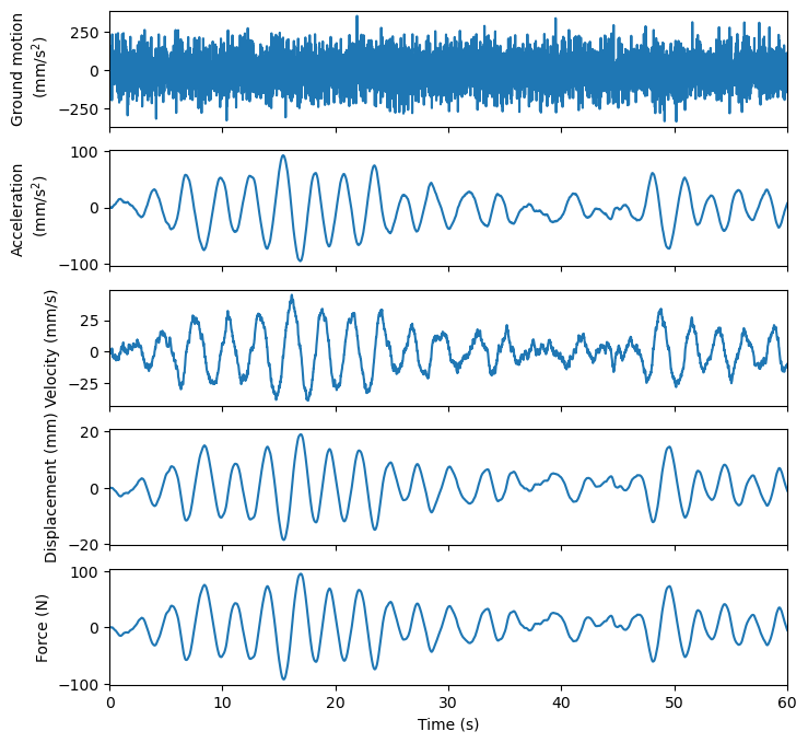
白噪声激励下结构响应
下面我们生成一段白噪声,并作为结构的基底加速度输入,来分析结构的响应。再通过响应的结果来判断 SDOF 的自振特性。
1 | # 白噪声激励下结构响应 |
Omega: 2.23606797749979
下面对结构的位移做傅里叶变换
1 | # 傅里叶变换 |
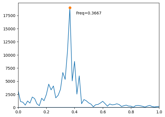
根据结构性质来计算结构的频率:
$$ f_n = \frac{\omega_n}{2\pi} = \frac{1}{2 \pi} \sqrt{\frac{k}{m}} = 0.3561 $$
$$ f_D = f_n / \sqrt{(1 - \zeta^2)} = 0.3565 $$
可见测得的频率与结构的自振频率接近,误差是采样频率导致的。