上一篇文章 使用 Pybind11 将 C++ 代码封装为 Python 库 介绍了 Pybind11 的使用方法。本文继续上一章的内容,在 OpenSees 的 C++ 源代码中,写一个单轴材料模型 UniaxialMaterial 滞回曲线的生成程序,并封装到 Python 库。
下载 OpenSees 源代码 首先在 Github 上将 OpenSees 下载下来。打开 OpenSees 官方源代码仓库 ,在写着 master 的下拉菜单中,将版本回退到最近的标签,我目前是 v3.5.0 ,再在右边写着 Code 的绿色按钮的下拉菜单中点击 Download zip ,则可以将 OpenSees 源代码下载到本地,解压即可。
考虑到使用 Windows 的用户比较多,这里使用 Visual Studio (VS) 来进行编译。我电脑中的 VS 是 Community 2019 版。
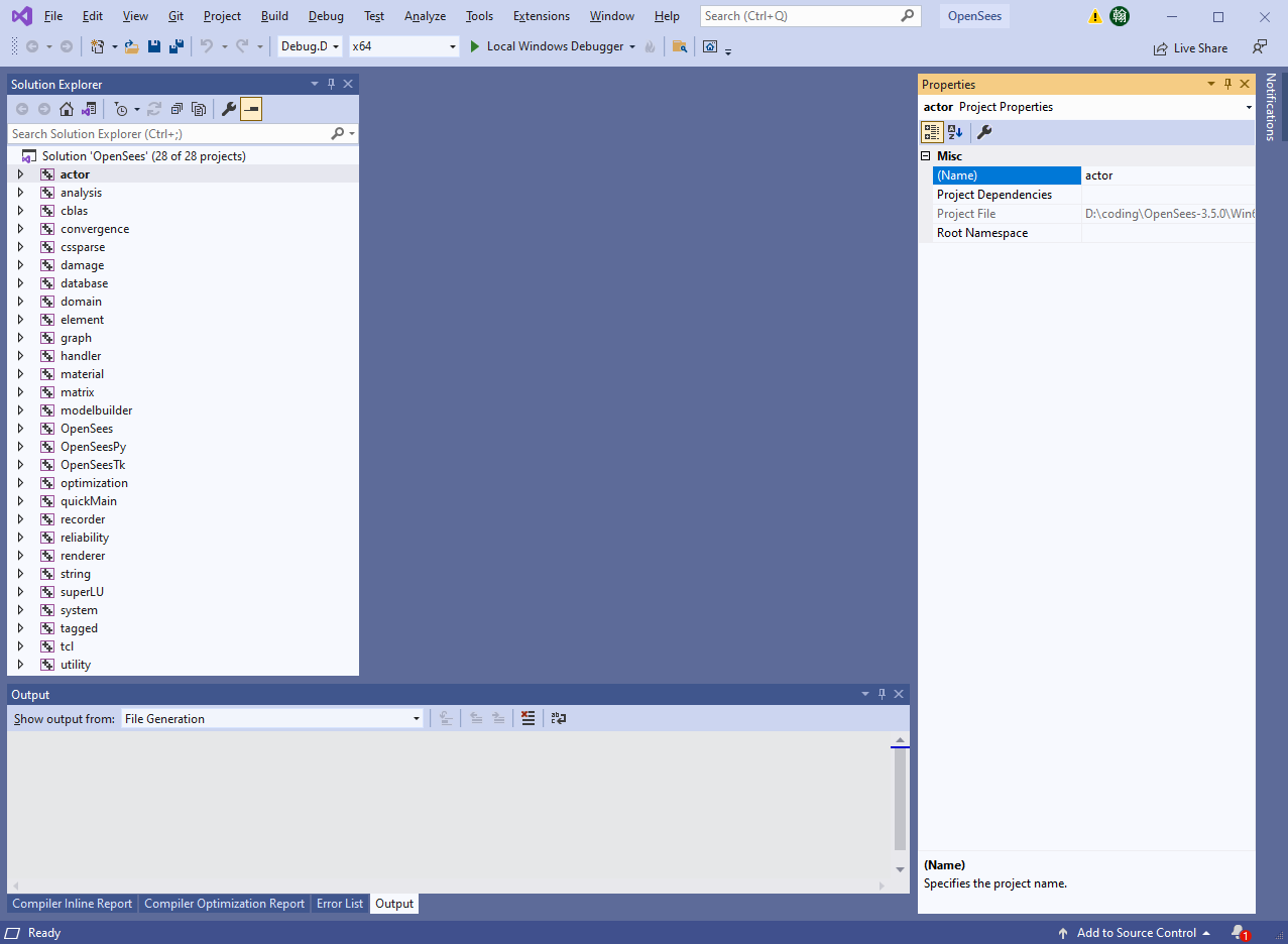
在 OpenSees 的源代码中,找到 Win64 ,打开后,有一个 OpenSees.sln 文件,即开发者为 OpenSees 创建的 VS 解决方案文件。双击该文件,即可唤起 VS ,打开的界面如图所示。
在这里面,可以很轻松地编译 OpenSees ,也可以自己开发新的代码。要想编译的话,只要在 OpenSees 对应的 Project 位置点击右键再 Build 即可。本文不讨论如何编译 OpenSees 了,如果有需要,可以看我的另一篇视频教程 编译 OpenSees 的方法 。
值得一提的是,历史上 OpenSees 在 Windows 中使用 VS 解决方案编译,在 Linux 和 Mac 中使用 make 编译。后来有了 CMake ,使不同平台可以统一。现在 OpenSees 可以通过 CMake 来编译了。然而我们这里使用的还是不借助 CMake 的老方法。
编译示例项目 很多读者没有注意到的是, OpenSees 除了可以使用 tcl 和 Python 两种语言作为解释器之外,还有一种使用方式是直接用 C++ 来调用,而且这种方式效率最高。在我的博文 OpenSees 不同解释器的性能比较 中对此进行过讨论。
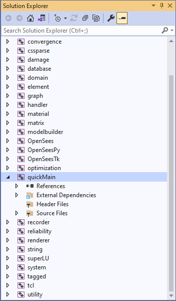
在当前打开的 VS 环境中,已经置入了一个使用 C++ 来调用 OpenSees 的示例,作为一个 Project ,它的名字叫 quickMain ,如图所示:
来看一下这个 Project 里面的内容。先看 References ,里面放入了一些其他的 Project 。 External dependencies 里面有一些头文件,是从 OpenSees 源代码中拿过来的。Source files 里面有三个文件,其中 main.cpp 文件存放了主要的代码。实际上,这个源文件位置不在 OpenSees 源代码的 SRC 中,而是在 EXAMPLES 文件夹下的 Example1 中。这个例子实现的是 OpenSees 的经典静力分析案例,可以在我的博文 OpenSees 不同解释器的性能比较 中看到这个代码实现的功能。
下面我们来尝试编译。首先在图标栏里,把 Debug 模式改为 Release 模式。然后在 quickMain 上点击右键,选择 Build ,很快报了如下错:
1
2
3
4
5
6
7
... 1>Generating Code... 1>LINK : warning LNK4075: ignoring '/INCREMENTAL' due to '/FORCE' specification 1>LINK : fatal error LNK1181: cannot open input file 'reliability.lib' 1>C:\Program Files (x86)\Microsoft Visual Studio\2019\Community\MSBuild\Microsoft\VC\v160\Microsoft.CppCommon.targets(1074,5): error MSB6006: "link.exe" exited with code 1181. 1>Done building project "quickMain.vcxproj" -- FAILED. ========== Build: 0 succeeded, 1 failed, 0 up-to-date, 0 skipped ==========
这里的提示为,链接器 LINKER 无法链接到名为 reliability.lib 文件。这说明,在 quickMain 这个 Project 中需要依赖其他 Project 生成的静态库文件。这些静态库文件我们还没有编译。
由于错误提示没有 reliability.lib ,我们就要思考两个问题。第一个是我们需不需要这个文件,第二个是我们如何找到这个文件。
reliability 其实是 OpenSees 中一个使用 FOAM 法分析可靠度的程序。在个简单的静力分析里面,其实并不需要这些功能。因此,对于这个报错,我们把对 reliability.lib 的链接需求给去掉。
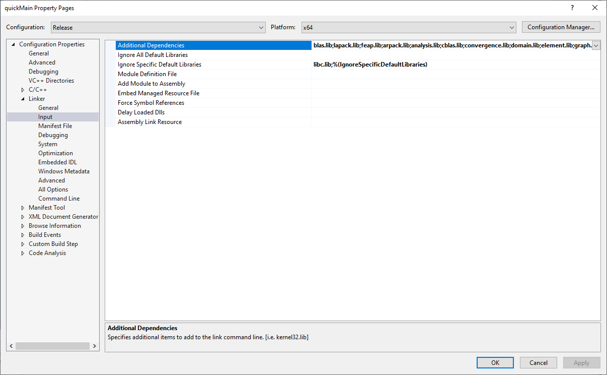
VS 的链接器需要链接哪些文件呢?在 quickMain 上点击右键,点击 Properties ,在弹出的菜单左侧选择 Linker 下的 Input ,可以看到右边第一行是 Additional Dependencies ,如图所示:
这里面列出了一系列的 Dependencies ,可以看到第一个就是 reliability.lib 。也就是说,刚才在编译的时候,链接器首先链接的就是这个文件,但是没有找到,所以就直接报错了。
我们看一下这个 Dependencies 列表:
1
2
3
4
5
6
7
8
9
10
11
12
13
14
15
16
17
18
19
20
21
22
23
24
25
26
27
reliability.lib database.lib blas.lib lapack.lib feap.lib arpack.lib analysis.lib cblas.lib convergence.lib domain.lib element.lib graph.lib material.lib matrix.lib modelbuilder.lib recorder.lib superLU.lib system.lib tagged.lib utility.lib ifconsol.lib libifcoremt.lib libmmt.lib odbc32.lib odbccp32.lib OpenGL32.lib glu32.lib
其中有一些明显用不上的,可以直接在这个列表里面删去,比如说上面的 reliability.lib 是分析可靠度的,database.lib 是用于数据库存储的,等等。当然,如果读者无法判断哪些 lib 可以删掉,也可以全部保留,只是会编译出很多无用的库来,浪费时间和空间。
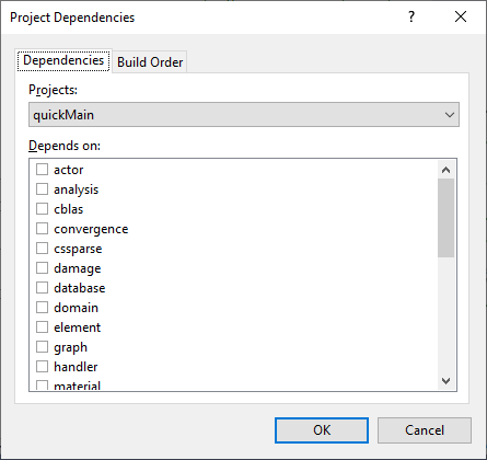
假设我们不去删掉 reliability.lib 这个依赖项,那么如何处理呢,就需要思考第二个问题,如何找到这个文件。实际上,这个文件是 reliability 这个项目编译得到的。因此我们需要编译 reliability 这个项目。下面我们在 quickMain 上点击右键,找到 Build Dependencies (构建依赖)下面的 Project Dependencies (项目依赖),弹出如下图所示的对话框:
我们就把 reliability 这个项目加上。然后再编译,可以看到,VS 先编译了 reliability 这个模块。但是在编译这个模块的过程中,又发生了错误,有如下错误代码:
1
2
3
4
5
6
... 1>CurvatureFitting.cpp 1>D:\coding\OpenSees-3.5.0\src\optimization\domain\component\DesignVariable.h(39,10): fatal error C1083: Cannot open include file: 'tcl.h': No such file or directory 1>CurvaturesBySearchAlgorithm.cpp 1>D:\coding\OpenSees-3.5.0\src\optimization\domain\component\DesignVariable.h(39,10): fatal error C1083: Cannot open include file: 'tcl.h': No such file or directory ...
提示很清楚,找不到 tcl.h 。实际上,tcl 作为一个解释器,不应该出现在编译源代码的时候,而应该解耦开。但是可能有很多历史原因,他们被写在了一起。所以这里,我们要告诉 VS ,在哪里可以找到这个头文件。
我的电脑里面安装的是 miniconda ,也就是 anaconda 的缩减版本,它自带有 tcl 不用额外安装了。这个 tcl.h 文件就在安装目录下的 Library 里面的 include 里面。我电脑上的绝对路径为 C:\Users\hanli\miniconda3\Library\include 。
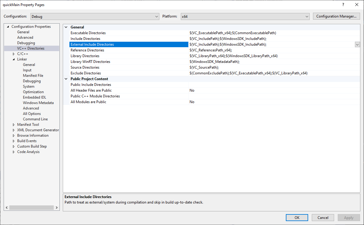
在 reliability 上点击右键,打开 Properties ,左侧选 VC++ Directories ,右侧可以看到一个 External Include Directories ,如下图所示 。点击右面的下拉箭头,再点击 Edit ,将上面的路径添加进来。
然后再进行编译,可以发现,不再报 reliability.lib 的错了,而是报其他库的错。这时我们就可以用类似的方法去解决其他报错的问题了。
由于很多 Project 都要用到 tcl.h ,都去修改比较麻烦。这里我把所有 tcl 开头的头文件复制到 SRC 文件夹里,这是一个检索路径,就不用再逐一添加检索路径了。
还有一个错误提示,是 ifconsol.lib ,这个是与 Fortran 有关的库。这个可以通过安装 Intel oneAPI 来完成。在我的电脑里,它的路径是 C: \ Program Files (x86) \ Intel \ oneAPI \ compiler \ latest \ windows \ compiler \ lib \ intel64_win 。可以把这个路径加到 Properties 里面 Linker - General - Additional Linker Directories 里面。
持续添加 Build dependencies ,直到最终报 success ,没有 fail 为止。
这个成功编译的文件在哪里呢?可以看 quickMain 的 Properties 里面的 Output Directory ,可以看出是在 OpenSees 中的 bin 文件夹。打开后,可以找到名为 quickMain.exe 的可执行文件。
打开 PowerShell 终端,键入 ./quickMain 可以看到示例 C++ 代码被成功执行了。
用 C++ 写 OpenSees 程序 由于直接使用 C++ 写函数没有完善的文档,只能通过阅读源代码的方式实现。还好的是源代码中的注释还算清晰。下面我们在 main.cpp 的基础上进行修改。
示例代码只使用了 Truss 单元,所以只引入了 Truss.h 这个头文件。我们想使用 twoNodeLink 这个单元,就要去找对应的头文件。在 Element 文件夹里面可以找到 twoNodeLink 这个文件夹,下面有 twoNodeLink.h 这个文件。那么在代码中引入这个头文件就可以了。类似地,还要引入 Displacement Control 相关,还有 Constraints 相关的头文件。原来的 Constraints 用的是 Panelty ,这里我们给改成 Transformation 。现在的头文件为:
1 2 3 4 5 6 7 8 9 10 11 12 13 14 15 16 17 18 19 20 21 22 23 24 25 26 27 28 29 30 #include <stdlib.h> #include <OPS_Globals.h> #include <StandardStream.h> #include <ArrayOfTaggedObjects.h> #include <Domain.h> #include <Node.h> #include <Truss.h> #include <twoNodeLink\TwoNodeLink.h> #include <ElasticMaterial.h> #include <SP_Constraint.h> #include <LoadPattern.h> #include <LinearSeries.h> #include <NodalLoad.h> #include <StaticAnalysis.h> #include <AnalysisModel.h> #include <Linear.h> #include <PenaltyConstraintHandler.h> #include <TransformationConstraintHandler.h> #include <DOF_Numberer.h> #include <RCM.h> #include <LoadControl.h> #include <DisplacementControl.h> #include <BandSPDLinSOE.h> #include <BandSPDLinLapackSolver.h>
首先我们先进行一次一步加载来测试一下,代码如下:
1
2
3
4
5
6
7
8
9
10
11
12
13
14
15
16
17
18
19
20
21
22
23
24
25
26
27
28
29
30
31
32
33
34
35
36
37
38
39
40
41
42
43
44
45
46
47
48
49
50
51
52
53
54
55
void test_cyclic () Domain* theDomain = new Domain (); Node* node0 = new Node (1 , 1 , 0.0 ); Node* node1 = new Node (2 , 1 , 0.0 ); theDomain->addNode (node0); theDomain->addNode (node1); SP_Constraint* sp1 = new SP_Constraint (1 , 0 , 0.0 ); theDomain->addSP_Constraint (sp1); UniaxialMaterial* theMaterial = new ElasticMaterial (1 , 3000 ); int directions[1 ] = { 0 }; const ID* id_dir = new ID (directions, 1 ); TwoNodeLink* ele = new TwoNodeLink (1 , 1 , 1 , 2 , *id_dir, &theMaterial); theDomain->addElement (ele); TimeSeries* theSeries = new LinearSeries (); LoadPattern* theLoadPattern = new LoadPattern (1 ); theLoadPattern->setTimeSeries (theSeries); theDomain->addLoadPattern (theLoadPattern); Vector theLoadValues (1 ) ; theLoadValues (0 ) = 7.0 ; NodalLoad* theLoad = new NodalLoad (1 , 2 , theLoadValues); theDomain->addNodalLoad (theLoad, 1 ); AnalysisModel* theModel = new AnalysisModel (); EquiSolnAlgo* theSolnAlgo = new Linear (); StaticIntegrator* theIntegrator = new DisplacementControl (2 , 0 , 0.1 , theDomain, 1 , 0.1 , 0.1 ); ConstraintHandler* theHandler = new TransformationConstraintHandler (); RCM* theRCM = new RCM (); DOF_Numberer* theNumberer = new DOF_Numberer (*theRCM); BandSPDLinSolver* theSolver = new BandSPDLinLapackSolver (); LinearSOE* theSOE = new BandSPDLinSOE (*theSolver); StaticAnalysis theAnalysis (*theDomain, *theHandler, *theNumberer, *theModel, *theSolnAlgo, *theSOE, *theIntegrator) int numSteps = 1 ; theAnalysis.analyze (numSteps); const char * response = "forces" ; const Vector* theForces = theDomain->getElementResponse (1 , &response, 1 ); opserr << *theDomain; opserr << theForces[0 ]; theAnalysis.clearAll (); theDomain->clearAll (); delete theDomain; delete theMaterial; }
只要用过 OpenSees ,这里的大多数代码都很好理解。唯独在使用 TwoNodeLink 这个类的时候,有个 ID* 类型的 direction 变量要输入。由于 twoNodeLink 单元支持多种维度,所以这里肯定是支持一次型输入多维度的。但是本例中只有一个维度。如何处理,需要从 ID 这个类的定义中找答案。打开 ID 类的定义,它的构造函数有如下几个:
1
2
3
4
5
ID ();ID (int );ID (int size, int arraySize);ID (int *data, int size, bool cleanIt = false );ID (const ID &);
再结合后面的实现,可以推断出,这个类是用于保存一组 ID 的,所以变量名叫 directions 应该会更贴切一些。这里我们使用第四个构造函数,即指定了一个 size 为 1 的整数数组,里面的元素为第一个自由度,即 { 0 } 。然后构造 id_dir 实例,传入 twoNodeLink 中。其他用法也与这里类似,某个函数或方法不知道怎么用的时候,按住 ctrl 键再点击它,就可以追踪到相应的定义了。
当前这段代码想要运行的话,还要写一个 main 函数。并把原来的 main 函数注释掉。
1
2
3
int main () cyclic (); }
编译运行,就可以看到控制台上输出的信息了。
获取材料滞回曲线的函数 下面我们来修改这个函数,使之可以获取材料的滞回曲线。这个函数的主要功能是输入一系列材料参数,再输入一个位移控制的加载制度,输出对应的力。这里我们在一维空间中,使用一个 twoNodeLink 单元,挂在所需要的材料,再将单元的一端约束住,另一端进行位移控制加载。
这里我们使用 Steel01 材料,它有三个主要的材料参数。我们把这三个参数作为变量输入给函数。另外加载制度也可以作为变量输入给函数。需要的输出则是加载制度中每一个位移点对应的力。
这时的函数应该定义为:
1 std::vector<double > cyclic (std::vector<double > protocol, std::vector<double > params)
这里注意,在 OpenSees 中自行定义了一个叫 Vector 的类,它与我们这里使用的标准库 std 中的 vector 类是不同的。两个类实现的功能是差不多的, OpenSees 开发得比较早,可能是那个时候 std 库还不是很完善,所以进行了自定义。但是这里由于我们后面要与 Python 连接,使用 std 中的类可以使数据类型转换更方便。注意要引入头文件
下面先把 test_cyclic 中的弹性材料改为 Steel01 材料:
1 UniaxialMaterial* theMaterial = new Steel01 (1 , params[0 ], params[1 ], params[2 ]);
注意要在前面加上对 steel01.h 头文件的引用。
然后在分析中,需要使用一个循环,每一次分析 protocol 中的一步。
1 2 3 4 5 6 7 8 9 10 11 12 13 14 15 16 17 18 19 20 21 int protocol_size = protocol.size ();std::vector<double > result (protocol_size) ;double disp;int ok;bool success = true ;const char * response = "forces" ;for (int i = 0 ; i < protocol_size; i++) { disp = (i == 0 ) ? protocol[0 ] : protocol[i] - protocol[i - 1 ]; StaticIntegrator* theIntegrator = new DisplacementControl (2 , 0 , disp, theDomain, 1 , disp, disp); theAnalysis.setIntegrator (* theIntegrator); ok = theAnalysis.analyze (1 ); if (ok == 0 ) { const Vector* theForces = theDomain->getElementResponse (1 , &response, 1 ); result[i] = theForces[0 ][1 ]; } else { result[i] = 0.0 ; success = false ; } }
这段程序很简单,不过多解释了。下面写一个简单的测试,作为 main 函数:
1
2
3
4
5
6
7
8
9
10
int main () double protocol[12 ] = { 1. , 2. , 3. , 2. , 1. , 0. , -1. , -2. , -3. , -2. , -1. , 0. }; std::vector<double > vec_protocol (protocol, protocol + 12 ) ; double params[3 ] = { 233. , 123. , 0.1 }; std::vector<double > vec_params (params, params + 3 ) ; std::vector<double > res = cyclic (vec_protocol, vec_params); for (int i = 0 ; i < res.size (); i++) { opserr << res[i] << "\n" ; } }
编译运行,可以看到控制台中打印出了结果。
批量获取滞回曲线 下面我们给定一个加载制度,但是有不同的材料参数,来同时获取所有材料的滞回曲线。
有两种方式,一种是就使用上面的代码,每次加载一个模型,反复进行。另一种方式是使用多个 twoNodeLink 单元并联,每个单元用一套材料参数。我们先写后一种的代码,然后与前一种比较一下,看二者的效率是否有不同。
新建一个函数,函数头为:
1 std::vector<double > cyclic_batch (std::vector<double > protocol, std::vector<double > params)
这里我们默认 params 每个材料有三个参数,多个材料按三个三个连续排列。
在创建材料和单元时,需要用到一个循环:
1
2
3
4
5
6
7
const int NUM_MAT = 3 ;int mat_size = params.size () / NUM_MAT;for (int i = 0 ; i < mat_size; i++) { UniaxialMaterial* theMaterial = new Steel01 (1 , params[i * NUM_MAT], params[i * NUM_MAT + 1 ], params[i * NUM_MAT + 2 ]); TwoNodeLink* ele = new TwoNodeLink (1 , 1 , 1 , 2 , *id_dir, &theMaterial); theDomain->addElement (ele); }
然后在分析的部分,每一步产生的 Response 需要都保存起来。
1 2 3 4 5 6 7 8 9 10 11 12 13 std::vector<double > result (protocol_size * mat_size) ;if (ok == 0 ) { for (int j = 0 ; j < mat_size; j++) { const Vector* theForces = theDomain->getElementResponse (j + 1 , &response, 1 ); result[j * protocol_size + i] = theForces[0 ][1 ]; } } else { for (int j = 0 ; j < mat_size; j++) { result[j * protocol_size + i] = 0.0 ; } success = false ; }
再把测试用的 main() 函数修改一下:
1
2
3
4
5
6
7
8
9
10
11
12
int main () double protocol[12 ] = { 1 , 2 , 3 , 2 , 1 , 0 , -1 , -2 , -3 , -2 , -1 , 0 }; Vector vec_protocol; vec_protocol.setData (protocol, 12 ); double params[6 ] = { 233 , 123 , 0.1 , 12 , 13 , 0.2 }; Vector vec_params; vec_params.setData (params, 6 ); Vector c = cyclic_batch (vec_protocol, vec_params); for (int i = 0 ; i < c.Size (); i++) { opserr << c (i) << "\n" ; } }
编译运行,发现两套材料参数都输出来了。
把示例项目封装为 Python 库 下面我们把示例项目封装为 Python 库,以通过 Python 来调用。这里我们使用 Pybind11 来完成。在我的上一篇博文 使用 Pybind11 将 C++ 代码封装为 Python 库 中已经对 Pybind11 的使用方法进行了介绍。
首先将 Pybind11 的代码直接复制到项目 SRC 文件夹中,并在 main.cpp 中加入引用和命名空间:
1
2
3
4
#include <pybind11/pybind11.h> #include <Python.h> namespace py = pybind11;
注意要如果两个 include 报错的话,是因为编译器没有找到这两个头文件的位置,需要在 Properties 里面进行修改,在上一篇博文里面有介绍。
值得注意的是,在 Python 的 includes 文件夹里面也有名为 Node.h 的头文件。所以这个文件夹要放在所有 additional includes 的最后,以使程序先找到正确的 Node.h 文件。
把两个函数共同封装在一个包 opstuils 里面,要写的宏如下:
1
2
3
4
5
PYBIND11_MODULE (opsutils, m) { m.doc () = "Utility OpenSees functions." ; m.def ("cyclic" , &cyclic, "Cyclic tests for a single material" ); m.def ("cyclic_batch" , &cyclic_batch, "Cyclic tests for a batch of materials" ); }
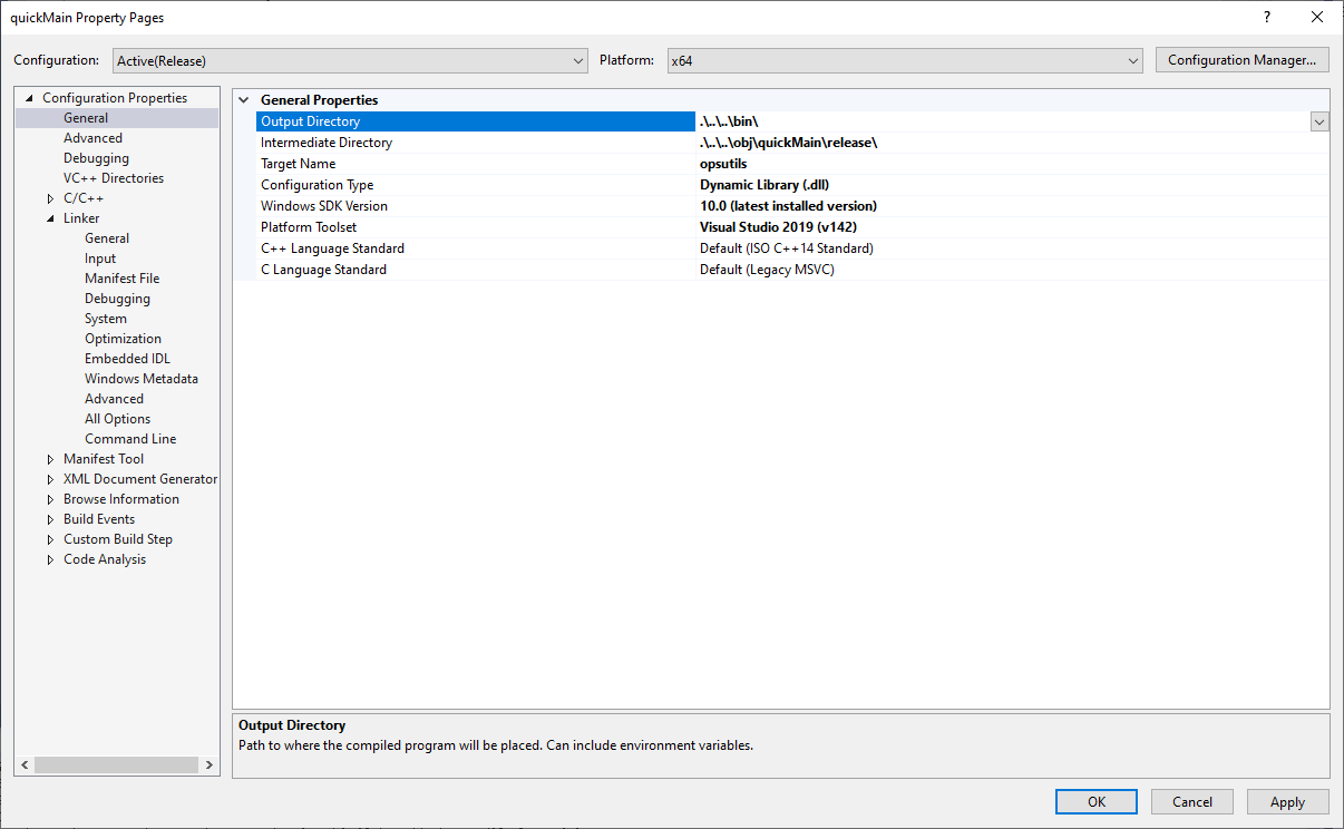
然后将项目的类型从可执行文件修改为动态链接库。方法为打开 quickMain Project 的 Properties, 将 Configuration Type 从 Application (.exe) 修改为 Dynamic Library (.dll) ,并在 Project Name 处指定一个名字,需要与上面的宏中第一个参数一致,为 opsutils ,界面如图所示。
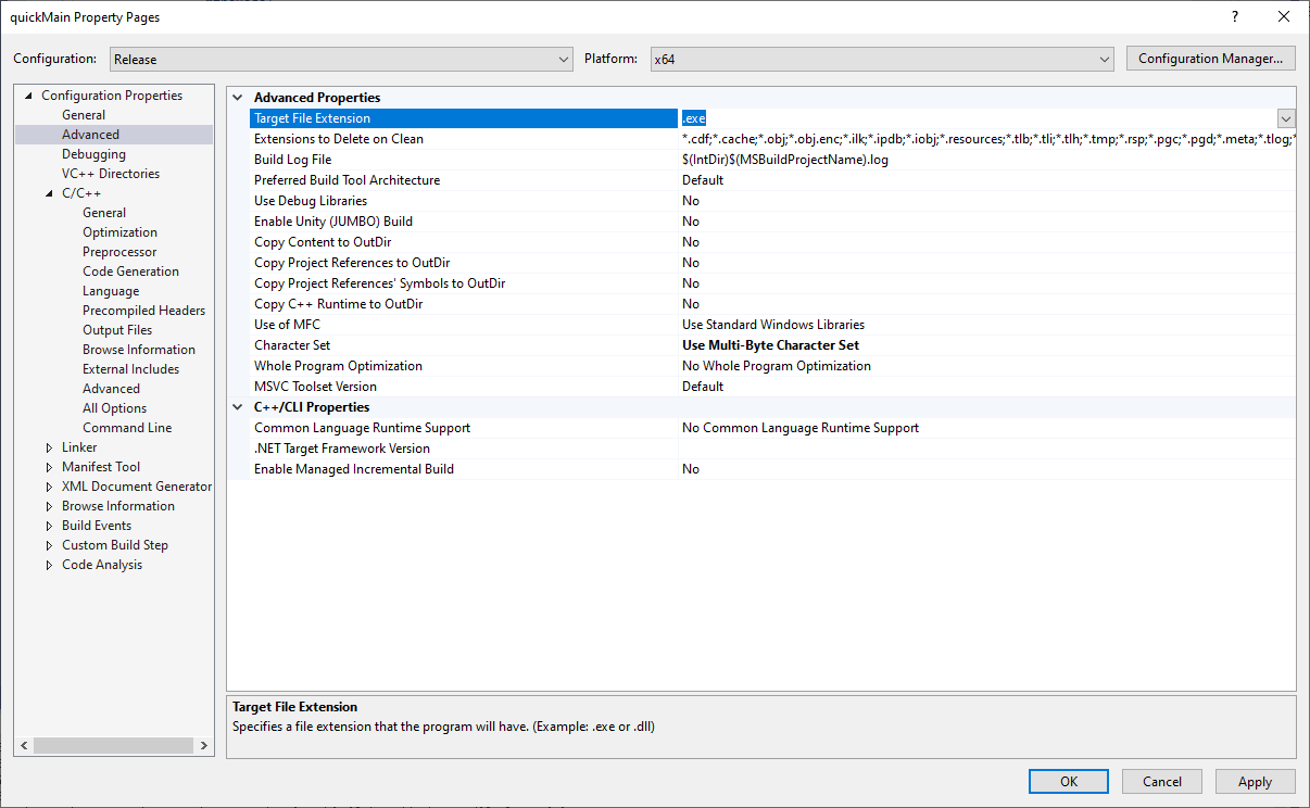
再到 Advanced 里面,把 Target File Extension 从 .exe 修改为 .pyd ,如图所示。
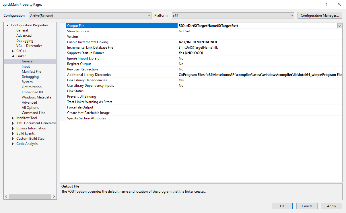
在 Linker 里面,有一个 Output File ,在当前这个项目中被设成了一个特殊值,我们这里改成默认值。
1 $(OutDir)$(TargetName)$(TargetExt)
编译,出现 LINKER 错误,找不到 Python38.lib ,这说明没有指定该文件所在的目录,需要到 Properties 中再指定一下。这在上篇博文中已经谈到了。添加好目录之后,再次编译,成功。
打开生成目录,可以看到有一个 opsutils.pyd 文件,只要这个文件在工作路径中,就可以使用刚才封装的函数了。打开终端测试一下:
1
2
3
4
5
>>> import opsutils as ou>>> ou.cyclic(... [1. , 2. , 3. , 2. , 1. , 0. , -1. , -2. , -3. , -2. , -1. , 0. ],... [233. , 123. , 0.1 ])[123.0 , 234.3 , 246.60000000000002 , 123.60000000000002 , 0.6000000000000227 , -122.39999999999998 , -222.00000000000003 , -234.3 , -246.60000000000002 , -123.60000000000002 , -0.6000000000000227 , 122.39999999999998 ]
Python 输出的结果与 C++ 输出的结果有细微的差别,可以看到 Python 在打印小数时,会跟很多0,并在最后有一点点浮动。这是由于浮点数的精度导致的。 C++ 在打印的时候自动帮助我们处理掉了这个问题,但是 Python 在打印的时候原封不动地进行了打印,所以只是打印的不同而已。实际上,如果在 C++ 中,把我们原来用于测试的 main() 函数输出为一个文件,并指定小数位数的话,得到的结果是与 Python 打印基本一致的。
1 2 3 4 5 6 7 8 9 10 #include <fstream> #include <iostream> #include <iomanip> ofstream fout; fout.open ("out.txt" ); for (int i = 0 ; i < res.size (); i++) { fout << std::fixed << std::setprecision (14 ) << res[i] << "\n" ; } fout.close ();
由于工程上我们不需要那么高的精度,所以这些差别都可以忽略了。
使用 OpsPy 写材料测试程序 下面我们把与 C++ 功能一模一样的程序使用 OpenSeesPy 来重新实现一遍。直接上代码
1
2
3
4
5
6
7
8
9
10
11
12
13
14
15
16
17
18
19
20
21
22
23
24
25
26
27
28
29
30
31
32
33
34
35
36
37
38
39
40
41
42
43
44
45
46
47
48
49
50
51
52
53
54
55
56
57
58
59
60
61
62
63
64
65
66
67
68
69
70
71
72
73
74
75
76
import openseespy.opensees as opsdef cyclic (protocol, params ): ops.model("basic" , "-ndm" , 1 , "-ndf" , 1 ) ops.node(1 , 0.0 ) ops.node(2 , 0.0 ) ops.fix(1 , 1 ) ops.uniaxialMaterial("Steel01" , 1 , params[0 ], params[1 ], params[2 ]) ops.element("twoNodeLink" , 1 , 1 , 2 , "-mat" , 1 , "-dir" , 1 ) ops.timeSeries("Linear" , 1 ) ops.pattern("Plain" , 1 , 1 ) ops.load(2 , 1.0 ) ops.algorithm("Newton" ) ops.integrator("DisplacementControl" , 2 , 1 , 1 ) ops.constraints("Transformation" ) ops.numberer("RCM" ) ops.system("BandSPD" ) ops.analysis("Static" ) protocol_size = len (protocol) result = [0. for i in range (protocol_size)] success = True for i in range (protocol_size): disp = protocol[i] if i == 0 else protocol[i] - protocol[i-1 ] ops.integrator("DisplacementControl" , 2 , 1 , disp) ok = ops.analyze(1 ) if ok == 0 : forces = ops.eleForce(1 ) result[i] = forces[1 ] else : success = False ops.wipe() return result def cyclic_batch (protocol, params ): ops.model("basic" , "-ndm" , 1 , "-ndf" , 1 ) ops.node(1 , 0.0 ) ops.node(2 , 0.0 ) ops.fix(1 , 1 ) NUM_MAT = 3 mat_size = len (params) // NUM_MAT for i in range (mat_size): ops.uniaxialMaterial("Steel01" , i + 1 , *params[i * NUM_MAT: i * NUM_MAT+3 ]) ops.element("twoNodeLink" , i + 1 , 1 , 2 , "-mat" , i + 1 , "-dir" , 1 ) ops.timeSeries("Linear" , 1 ) ops.pattern("Plain" , 1 , 1 ) ops.load(2 , 1.0 ) ops.algorithm("Newton" ) ops.integrator("DisplacementControl" , 2 , 1 , 1 ) ops.constraints("Transformation" ) ops.numberer("RCM" ) ops.system("BandSPD" ) ops.analysis("Static" ) protocol_size = len (protocol) result = [0. for _ in range (protocol_size * mat_size)] success = True for i in range (protocol_size): disp = protocol[i] if i == 0 else protocol[i] - protocol[i-1 ] ops.integrator("DisplacementControl" , 2 , 1 , disp) ok = ops.analyze(1 ) if ok == 0 : for j in range (mat_size): forces = ops.eleForce(j + 1 ) result[i + j * protocol_size] = forces[1 ] else : success = False ops.wipe() return result if __name__ == "__main__" : protocol = [1. , 2. , 3. , 2. , 1. , 0. , -1. , -2. , -3. , -2. , -1. , 0. ] params = [233. , 123. , 0.1 ] params2 = [ 233. , 123. , 0.1 , 12. , 13. , 0.2 ] print (cyclic(protocol, params)) print (cyclic_batch(protocol, params2))
性能比较 铺垫这么多,最激动人心的时刻到来了,那就是对比在 Python 中使用 C++ 封装代码的速度,以及使用 Python 版 OpenSees 的速度。
下面是用于测试的代码,计时借助 Jupyter 的 %time 魔法函数来完成。
先导入写好的几个函数
1
2
3
4
5
import randomfrom opspyutils import cyclic as py_cyclicfrom opspyutils import cyclic_batch as py_cyclic_batchfrom opsutils import cyclic as cpp_cyclicfrom opsutils import cyclic_batch as cpp_cyclic_batch
开始前先写一个给定加载制度,用于生成位移值的函数。 SmartAnalyze 中使用的就是类似的写法。
1
2
3
4
5
6
7
8
9
10
11
12
13
14
def create_protocol (target, step ): protocol = [] curr_disp = 0. for i, curr_target in enumerate (target): forward = True if i == 0 else (target[i] - target[i-1 ]) > 0 if forward: while curr_disp < curr_target: curr_disp += min (step, curr_target - curr_disp) protocol.append(curr_disp) else : while curr_disp > curr_target: curr_disp -= min (step, -(curr_target - curr_disp)) protocol.append(curr_disp) return protocol
然后来生成两个不同长度的 protocol 。
1
2
3
4
5
6
7
target1 = [2 , -2 , 4 , -4 , 6 , -6 , 8 , -8 , 10 , -10 , 0 ] step1 = 0.1 target2 = [5 , -5 , 10 , -10 , 15 , -15 , 20 , -20 , 25 , -25 , 30 , -30 , 35 , -35 , 40 , -40 , 50 , -50 , 0 ] step2 = 0.01 protocol1 = create_protocol(target1, step1) protocol2 = create_protocol(target2, step2) len (protocol1), len (protocol2)
可见两个 protocol 分别有约 1 千个点和 10 万个点。
材料参数我们先给一组,为确定下来的随机数。
1 mat1 = [9404 , 8090 , 0.2 ]
然后就可以揭晓分析时间了
1
2
%timeit py_cyclic(protocol1, mat1) %timeit cpp_cyclic(protocol1, mat1)
1
2
32.5 ms ± 6.27 ms per loop (mean ± std. dev. of 7 runs, 10 loops each) 25.6 ms ± 2.86 ms per loop (mean ± std. dev. of 7 runs, 10 loops each)
可以看出,分析的速度都还算快,封装 C++ 的速度要大于直接使用 OpenSeesPy 的速度。
再来看当 protocol 点数很多的情况:
1
2
%timeit py_cyclic(protocol2, mat1) %timeit cpp_cyclic(protocol2, mat1)
1
2
2.12 s ± 125 ms per loop (mean ± std. dev. of 7 runs, 1 loop each) 1.71 s ± 41.9 ms per loop (mean ± std. dev. of 7 runs, 1 loop each)
可见点数极多时,封装 C++ 的速度仍然比 Python 的速度快,与点数少时相似,都是提高 20% 左右。
下面我们使用 batch 来分析大量材料,这里使用 1 千个材料,并与单条分析来对比。首先使用 numpy 的 random 来创建随机材料参数:
1
2
3
4
5
6
import numpy as npbm1 = np.random.rand(1000 , 3 ) bm1[:, 0 ] *= 10000 bm1[:, 1 ] *= 10000 batch_mat1 = bm1.flatten().tolist()
然后要写个函数,实现用单个材料来计算多个材料
1
2
3
4
5
6
7
8
9
10
11
def py_cyclic_loop (protocol, mat, num=1000 ): results = [] for i in range (num): results += py_cyclic(protocol, mat[(i*3 ) : (i*3 + 3 )]) return results def cpp_cyclic_loop (protocol, mat, num=1000 ): results = [] for i in range (num): results += cpp_cyclic(protocol, mat[(i*3 ) : (i*3 + 3 )]) return results
然后来比较时间:
1
2
3
4
%timeit py_cyclic_batch(protocol1, batch_mat1) %timeit cpp_cyclic_batch(protocol1, batch_mat1) %timeit py_cyclic_loop(protocol1, batch_mat1) %timeit cpp_cyclic_loop(protocol1, batch_mat1)
1
2
3
4
10.2 s ± 781 ms per loop (mean ± std. dev. of 7 runs, 1 loop each) 8.09 s ± 195 ms per loop (mean ± std. dev. of 7 runs, 1 loop each) 1min 7s ± 27.1 s per loop (mean ± std. dev. of 7 runs, 1 loop each) 41.7 s ± 9.64 s per loop (mean ± std. dev. of 7 runs, 1 loop each)
可见使用 batch 分析的方法,效率要远远高于循环的方法。此外,在大量材料分析中,封装 C++ 的效率要略高于 OpenSeesPy 的效率。
封装优化 从前文可以看出,封装 C++ 并没有带来太大的效率提升。查阅 Pybind11 的文档,发现主要是因为使用自动的类型转换时,在 C++ 与 Python 之前的通信都是通过复制来完成的,这就造成了效率的降低。如果能直接从内存中传递参数,势必效率会有很大的提高。
查看 Pybind11 的文档,发现它支持一个数据类型 py::array_t<T> ,可以暴露给 Python 中的 numpy ,通过操作内存来运算。我们来尝试一下使用它来完成工作。
另外,原来的 cyclic_batch 能实现的功能其实已经包括了 cyclic 的全部功能。这里我们把它们整合起来,成为 cyclic2 。完整的代码如下:
1 2 3 4 5 6 7 8 9 10 11 12 13 14 15 16 17 18 19 20 21 22 23 24 25 26 27 28 29 30 31 32 33 34 35 36 37 38 39 40 41 42 43 44 45 46 47 48 49 50 51 52 53 54 55 56 57 58 59 60 61 62 63 64 65 66 67 68 69 70 71 72 73 74 75 76 77 78 79 80 81 82 83 84 85 86 87 88 89 90 91 92 93 94 95 96 py::array_t <double > cyclic2 (py::array_t <double > protocol, py::array_t <double > mats) { if (protocol.ndim () != 1 ) { throw std::runtime_error ("Protocol must in dimension 1." ); } auto p = protocol.mutable_unchecked<1 >(); py::ssize_t len_p = p.shape (0 ); py::buffer_info ptc = protocol.request (); if (mats.ndim () != 2 ) { throw std::runtime_error ("Material parameters must in dimension 2." ); } auto m = mats.mutable_unchecked<2 >(); py::ssize_t len_m = m.shape (0 ); py::ssize_t len_param = m.shape (1 ); if (len_param != 3 ) { throw std::runtime_error ("Number of parameters must be 3." ); } Domain* theDomain = new Domain (); Node* node0 = new Node (1 , 1 , 0.0 ); Node* node1 = new Node (2 , 1 , 0.0 ); theDomain->addNode (node0); theDomain->addNode (node1); SP_Constraint* sp1 = new SP_Constraint (1 , 0 , 0.0 ); theDomain->addSP_Constraint (sp1); int directions[1 ] = { 0 }; const ID* id_dir = new ID (directions, 1 ); std::vector<UniaxialMaterial>* mats = new std::vector<UniaxialMaterial>(len_m); for (int i = 0 ; i < len_m; i++) { UniaxialMaterial* theMaterial = new Steel01 (i + 1 , m (i, 0 ), m (i, 1 ), m (i, 2 )); TwoNodeLink* ele = new TwoNodeLink (i + 1 , 1 , 1 , 2 , *id_dir, &theMaterial); theDomain->addElement (ele); } TimeSeries* theSeries = new LinearSeries (); LoadPattern* theLoadPattern = new LoadPattern (1 ); theLoadPattern->setTimeSeries (theSeries); theDomain->addLoadPattern (theLoadPattern); Vector theLoadValues (1 ) ; theLoadValues (0 ) = 1.0 ; NodalLoad* theLoad = new NodalLoad (1 , 2 , theLoadValues); theDomain->addNodalLoad (theLoad, 1 ); AnalysisModel* theModel = new AnalysisModel (); EquiSolnAlgo* theSolnAlgo = new Linear (); StaticIntegrator* theIntegrator = new DisplacementControl (2 , 0 , 1.0 , theDomain, 1 , 1.0 , 1.0 ); ConstraintHandler* theHandler = new TransformationConstraintHandler (); RCM* theRCM = new RCM (); DOF_Numberer* theNumberer = new DOF_Numberer (*theRCM); BandSPDLinSolver* theSolver = new BandSPDLinLapackSolver (); LinearSOE* theSOE = new BandSPDLinSOE (*theSolver); StaticAnalysis theAnalysis (*theDomain, *theHandler, *theNumberer, *theModel, *theSolnAlgo, *theSOE, *theIntegrator) auto result = py::array_t <double >({ len_m, len_p }); auto r = result.mutable_unchecked<2 >(); double disp; int ok; bool success = true ; const char * response = "forces" ; for (int i = 0 ; i < len_p; i++) { disp = (i == 0 ) ? p (i) : p (i) - p (i-1 ); StaticIntegrator* theIntegrator = new DisplacementControl (2 , 0 , disp, theDomain, 1 , disp, disp); theAnalysis.setIntegrator (*theIntegrator); ok = theAnalysis.analyze (1 ); if (ok == 0 ) { for (int j = 0 ; j < len_m; j++) { const Vector* theForces = theDomain->getElementResponse (j + 1 , &response, 1 ); r (j, i) = theForces[0 ][1 ]; } } else { for (int j = 0 ; j < len_m; j++) { r (j, i) = 0.0 ; } success = false ; } } theAnalysis.clearAll (); theDomain->clearAll (); delete theDomain; return result; }
再来比较大批量计算的速度:
1
2
3
%timeit numpy_cyclic_batch(np.array(protocol1), bm1) %timeit py_cyclic_batch(protocol1, batch_mat1) %timeit cpp_cyclic_batch(protocol1, batch_mat1)
1
2
3
7.38 s ± 287 ms per loop (mean ± std. dev. of 7 runs, 1 loop each) 9 s ± 286 ms per loop (mean ± std. dev. of 7 runs, 1 loop each) 7.79 s ± 312 ms per loop (mean ± std. dev. of 7 runs, 1 loop each)
可以看到,使用新的封装方式,比使用原来的封装方式的速度又提升了一些。